10. Simulation visualization

Topics: Plotting, Mesh visualization

The corresponding python script: STEPS_Tutorial_Visual.py

In a previous chapter, we introduced how to save data to HDF5 files and generate XDMF files in order to visualize the data in the Paraview software.

In this chapter, we will use the STEPS visualization toolkit to interactively visualize STEPS simulations. To demonstrate this, we will use the simple IP3 receptor model introduced in the surface-volume reactions chapter. The STEPS visualization toolkit was originally described in the following article: Python-based geometry preparation and simulation visualization toolkits for STEPS.

A full decription of all available classes and functions is available in the API reference page.

10.1. Prerequisites

The following third-party python packages are required to use the visualization toolkit.

1. NumPy

2. PyQt

3. PyQtGraph

10.2. IP3 receptor model visualization

10.2.1. Biochemical model

We will use a spatial extension of the IP3 receptor model that we used in a previous chapter. The main difference consists in adding diffusion rules for Ca and IP3:

import steps.interface

from steps.model import *
from steps.geom import *
from steps.rng import *
from steps.sim import *
from steps.saving import *
from steps.visual import *

# Source:
#   Allbritton, N.L., Meyer, T., and Stryer, L. (1992).
#   Range of messenger action of calcium ion and inositol
#   1,4,5-triphosphate. Science 258, 1812-1815.
DCST_Ca = 0.065e-9
DCST_IP3 = 0.283e-9

mdl = Model()
r = ReactionManager()

with mdl:
    # chemical species objects
    Ca, IP3, R, RIP3, Ropen, RCa, R2Ca, R3Ca, R4Ca = Species.Create()

    ssys = SurfaceSystem.Create()
    with ssys:
        # IP3 and activating Ca binding
        R.s    + IP3.o <r[1]> RIP3.s
        RIP3.s + Ca.o  <r[2]> Ropen.s
        r[1].K = 1000000000.0, 25800.0
        r[2].K = 8000000000.0, 2000.0

        # Inactivating Ca binding
        R.s    + Ca.o <r[3]> RCa.s
        RCa.s  + Ca.o <r[4]> R2Ca.s
        R2Ca.s + Ca.o <r[5]> R3Ca.s
        R3Ca.s + Ca.o <r[6]> R4Ca.s
        r[3].K = 8889000.0, 5.0
        r[4].K = 20000000.0, 10.0
        r[5].K = 40000000.0, 15.0
        r[6].K = 60000000.0, 20.0

        # Ca ions passing through open IP3R channel
        Ca.i + Ropen.s <r[1]> Ropen.s + Ca.o
        # Corresponds to Ca input ~ 20000/ms for open receptor
        r[1].K = 8000000.0, 8000000.0

    vsys = VolumeSystem.Create()
    with vsys:
        # Create diffusion rules
        Ca_diff =  Diffusion.Create(Ca,  DCST_Ca)
        IP3_diff = Diffusion.Create(IP3, DCST_IP3)

We then load the tetrahedral mesh from file. This mesh already contains the patch and the compartments that were declared in the original IP3R model. We will then create the corresponding simulation object, and initialize the simulation:

mesh = TetMesh.Load('meshes/ip3r_mesh')

# Create random number generator
rng = RNG('mt19937', 512, 456)

# Create reaction-diffusion solver object
sim = Simulation('Tetexact', mdl, mesh, rng)

sim.newRun()

# Setup initial condition
sim.cyt.Ca.Count = 1
sim.cyt.IP3.Conc = 2.5e-06
sim.ER.Ca.Conc = 0.00015
sim.memb.R.Count = 16

rs = ResultSelector(sim)

Model checking:
No errors were found

In contrast with other chapters, we declare a ResultSelector object but we will not save any data with it. It will instead be used to describe which data we want to plot.

10.2.2. Declaring visualization elements

The next step is to describe what we want to display:

# Create control
sc = SimControl(end_time = 1.0, upd_interval = 0.0001)

with sc:
    # Plots
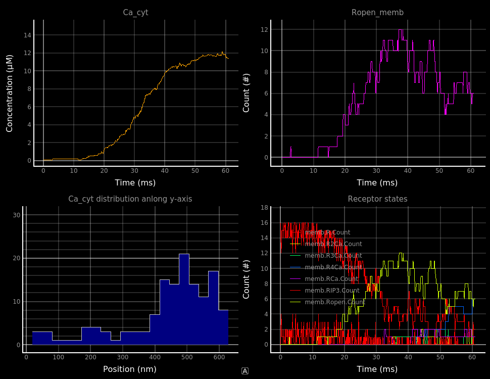
    plots_d = PlotDisplay('IP3 Receptor Model')
    with plots_d:

        TimePlot(rs.cyt.Ca.Conc,
            title='Ca_cyt',
            pen=(255, 0.647 * 255, 0),
            data_size=1000,
            y_range=[0, 15e-6],
            y_label=('Concentration', 'M')
        )

        TimePlot(rs.memb.Ropen.Count,
            title='Ropen_memb',
            pen=(255, 0, 255),
            data_size=1000,
            y_range=[0, 10],
            y_label=('Count', '#')
        )

        NewRow()

        SpatialPlot(rs.TETS(mesh.cyt.tets).Ca.Count,
            title='Ca_cyt distribution anlong y-axis',
            axis=[0, 1, 0],
            y_range=[0, 30]
        )

        TimePlot(rs.memb.MATCH('R.*').Count,
            title='Receptor states',
            data_size=1000,
            y_range=[0, 17],
            y_label=('Count', '#')
        )

    # 3D displays
    ER_d, CytIP3_d, CytCa_d, memb_d, full_d = SimDisplay.Create(
        'ER', 'Cyt IP3', 'Cyt Calcium', 'memb', 'Full view'
    )

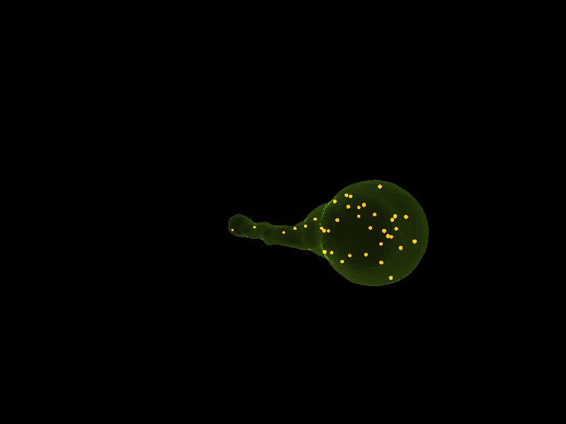
    with ER_d:
        # Static mesh element
        ElementDisplay(rs.ER, color=[0.678, 1, 0.184, 0.05])
        # Dynamic element
        ElementDisplay(rs.ER.Ca, color=[1, 0.647, 0, 1], spec_size = 0.005)

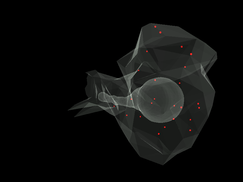
    with CytIP3_d:
        ElementDisplay(rs.cyt, color=[0.941, 1, 0.941, 0.05])
        ElementDisplay(rs.cyt.IP3, color=[1, 0, 0, 1], spec_size = 0.005)

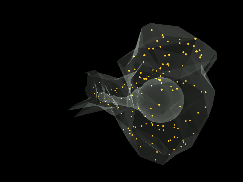
    with CytCa_d:
        ElementDisplay(rs.cyt, color=[0.941, 1, 0.941, 0.05])
        ElementDisplay(rs.cyt.Ca, color=[1, 0.647, 0, 1], spec_size = 0.005)

    with memb_d:
        ElementDisplay(rs.memb, color=[1, 0.973, 0.863, 0.05])

        # Different colors depending on receptor state
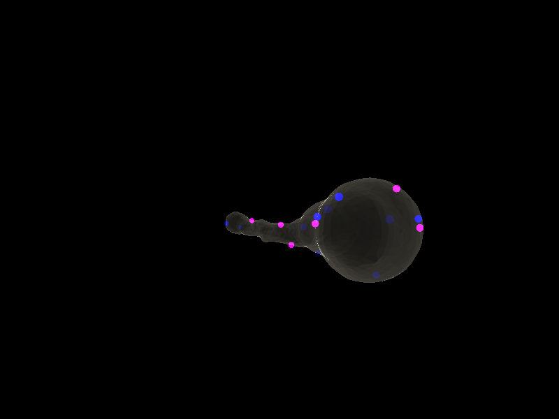
        spec2Col = {"R" : [0.0, 0.0, 1.0, 1.0], "RIP3" : [1.0, 0.0, 1.0, 0.2],
            "Ropen" : [1.0, 0.0, 1.0, 1.0], "RCa" : [0.0, 0.0, 1.0, 0.8],
            "R2Ca" : [0.0, 0.0, 1.0, 0.6], "R3Ca" : [0.0, 0.0, 1.0, 0.4],
            "R4Ca" : [0.0, 0.0, 1.0, 0.2]
        }
        ElementDisplay(
            rs.memb.MATCH('R.*'), spec_size = 0.01,
            color=lambda spec: spec2Col[spec.name]
        )

    # Merge all sub-displays to the full one
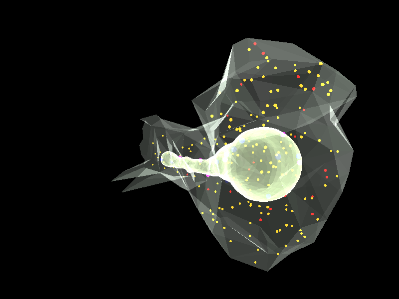
    full_d.merge(ER_d, CytIP3_d, CytCa_d, memb_d)

# Enter visualization loop
sc.run()

In order to visualize our simulation, we create a SimControl object which represents the simulation control window and will be used to group all other windows. These latter need to be declared inside the with sc: block, in the same way as compartments are declared in a with mesh: block.

After having declared all display windows, we need to launch the simulation with sc.run(). It is worth noting that the simulation object itself should not be controlled explicitely, it will be controlled by the simulation control window.

There are two types of display windows that can be used:

• Plot displays that contain plots showing the time evolution or spatial distribution of chosen quantities ; they are created with the PlotDisplay class

• Simulation displays that show 3D representations of the tetrahedral mesh with point representation of species ; they are created with the SimDisplay class

In this guide, we will introduce how to create and populate these windows but we will not describe in details all their parameters, more information can be found in the corresponding API reference page.

10.2.3. Plotting data

A plot display window is created by constructing a PlotDisplay object, it takes a string corresponding to the window title as first parameter. Sub-elements in the window are then declared inside a with block that uses the display window:

with sc:
    # PlotDisplays need to be declared in a SimControl
    plotWin = PlotDisplay('My title')
    with plotWin:
        # Declare plots
        # ...

There are then two types of plots that we can add to the plot display:

• Time plots showing the time evolution of chosen quantities ; they are created with the TimePlot class

• Spatial plots that can be used to display concentration gradients across space ; they are created with the SpatialPlot class

10.2.3.1. Time plots

In order to declare time plots, we need to provide at least one parameter to the TimePlot constructor: a result selector path to the data that should be plotted. The following code plots the same data as our main example, but without any of the optional formatting parameters:

with sc:
    # ...
    with plots_d:
        TimePlot(rs.cyt.Ca.Conc)
        TimePlot(rs.memb.Ropen.Count)
        # ...
        TimePlot(rs.memb.MATCH('R.*').Count)
    # ...

Note that, in contrast with conventional data saving, we do not need to add these result selectors to the simulation with the toSave method. It is possible to plot several lines in the sane TimePlot by passing a result selector path that encompasses several values. This is the case for the 3rd TimePlot in which we want to plot the count of IP3 receptors for each of its possible states.

In the main example, several formatting keyword arguments are used to set the plot title (title=...), set the color of the lines (pen=...), limit the amount of data that can be displayed at a time (data_size=...), set the range of the y-axis (y_range=...), and set the label of the y-axis (y_label=...). Additional formatting parameters are described in the API reference page.

10.2.3.2. Spatial plots

Spatial plots can be used to display the spatial distribution of some species along an axis. The following code corresponds to the same data as the main example, but without any of the optional parameters:

with sc:
    # ...
    with plots_d:
        SpatialPlot(rs.TETS(mesh.cyt.tets).Ca.Count, axis=[0, 1, 0])

The first parameter of the SpatialPlot constructor needs to be a result selector built using TETS(...) for tetrahedrons or TRIS(...) for triangles. For each of the tetrahedrons, it will query the corresponding value (number of ‘Ca’ here) and bin them according to the spatial location of the tetrahedron. The barycenter of the tetrahedrons is projected on the axis vector given as parameter. In our example, we project the locations on the [0, 1, 0] vector, i.e. the y axis. The locations are then binned into a number of bins that can be set with the nbins keyword parameter; its default value is 20.

The spatial plot can then operate in two different modes, that can be selected with the mode keyword parameter:

• ‘distr’, the default mode, for which the values associated with each tetrahedrons are being summed in each bin. When used with a .Count result selector, the resulting plot shows the distribution of species projected on the axis.

• ‘mean’, for which the values associated with each tetrahedrons are being averaged in each bin. When used with a .V result selector, the resulting plot shows the average electrical potential projected on the axis.

Additional formatting parameters are described in the API reference page.

10.2.3.3. Layout

Plots are added on a row from left to right, when NewRow() is called, a new row is created and subsequent plots will be added to this new row.

10.2.4. Visualizing mesh elements

Mesh elements are displayed in simulation display windows which are created by constructing a SimDisplay object. Mesh elements are then attached to the window by declaring them inside a with block that uses the simulation window:

with sc:
    # ...
    simWin = SimDisplay.Create('My title')
    with simWin:
        ElementDisplay(rs.compA)
        ElementDisplay(rs.compA.specB)
    # ...

In this example, we create a simulation window that will display the compA compartment as well as all specB species in this compartment. The surface of the compartment will be displayed in the window and the species will be represented as points. Note that compartments, patches, or simulation objects (species, channels, etc.) are all added to a simulation window with the same ElementDisplay class.

10.2.4.1. Setting the color of elements

In our main example, we use the color=... keyword parameter to set the colors of both compartments and species. Note that it takes a 4 elements list [r, g, b, a] with r, g, and b the colors itself (with each component being between 0 and 1) and a the alpha / transparency level, 0 meaning fully transparent and 1 fully opaque.

The color=... keyword parameter can also take a function, as is the case in our main example for displaying the different receptor states. The lambda function we use there takes a specie as parameter and returns a color as a 4 elements list.

The same thing can be done for setting the color of complexes according to their state. By default, if an element display is created with a path pointing to a complex, all states of the complex will be displayed in the same color. If the color=... keyword parameter is a function, it should take a complex state as parameter and return a color.

10.2.4.2. Addtional formatting parameters

The size of dots used to represent species can be adjusted with the spec_size=... keyword parameter. Additional keyword parameters are described in the API reference.

10.3. Screenshots

The following images correspond to the IP3 receptor example we presented in this chapter. They illustrate the different type of visualizations that are available in STEPS:

10.3.1. PlotDisplay - TimePlot and SpatialPlot

10.3.2. SimDisplay - ElementDisplay

10.3.2.1. Calcium in cytosol

10.3.2.2. Calcium in ER

10.3.2.3. IP3 in cytosol

10.3.2.4. IP3 receptors on ER surface

10.3.2.5. Combined view

10.3.3. SimControl