5. Diffusion in volumes and on surfaces

Topics: Volume diffusion, Surface diffusion, Diffusion boundaries, Tetrahedral mesh loading, Geometrical elements manipulation, Spatial data saving, Metadata saving.

The corresponding python script: STEPS_Tutorial_Diffusion.py

This chapter introduces how to model and simulate diffusion systems. First we will look at how to describe the diffusive motion of molecules by using object of class steps.model.Diffusion, then how to import a tetrahedral mesh by using the steps.geom.TetMesh class, then how to restrict the diffusion of species with diffusion boundaries, and finally how to use the 'Tetexact' solver in a simulation.

We will also familiarize ourselves with the manipulation of geometrical elements (tetrahedrons, triangles, etc.) and we will see how to save data in a 3D simulation and how to use matplotlib to visualize it.

5.1. Preliminary explanations

5.1.1. Diffusion in volumes

In reaction-diffusion simulations, each individual tetrahedron behaves like a well-mixed compartment where reactions can take place. Diffusive flux between tetrahedral elements is represented by a series of first-order reactions with rate constants derived from the local geometry and the diffusion constant parameter. Thus, STEPS can simulate full reaction-diffusion systems in complex geometries, but in this introduction we will start with a simple diffusion system.

We will simulate diffusion of a molecular species from a point source in an infinite volume, a problem chosen for simplicity and with a known analytical solution we can compare to our STEPS simulation results. As the volume in STEPS must of course be finite we will create a large mesh, inject our molecules into the central tetrahedron (as there is no concept of a point source in STEPS) and compare our results to the analytical solution up to a time when there are zero or an insignificant number of boundary events.

To compare our mean results in STEPS to an analytical solution we must solve the diffusion equation for one spatial dimension, the radial distance from the point source. The problem is simplified to one dimension because the symmetry of the problem dictates that, in the deterministic limit, the concentration at any given radial distance r from the point source will be equal at all points in space forming a two-dimensional “shell” at that r.

If all molecules exist at a single point at time 0, within an infinite boundary, the analytical solution is (see e.g. Crank, J. (1975) The Mathematics of Diffusion. Oxford: Clarendon Press):

\begin{equation} C(r,t)=\frac{N}{8(\pi Dt)^{3/2}}\exp\left(\frac{-r^{2}}{4Dt}\right) \end{equation}

where C is the concentration (if length units are meters the units of C are number of molecules/ \(m^{\text{3}}\)) at radial distance r from source at time t, N is the total number of injected molecules and D is the diffusion constant (in units \(m^{\text{2}}/s\)) .

5.1.2. Diffusion on surfaces

In STEPS, surface diffusion means movement of molecules between triangle elements within a patch and is used to model e.g. mobility of surface receptors within membranes.

In practice, simulating diffusion in surfaces is analogous to simulating diffusion in volumes, replacing volume system with surface system and compartment with patch. Here, we will demonstrate the simple case of free diffusion from a source on a large circular surface, which is somewhat analogous to free diffusion in a volume. In order to have both types of diffusion in the same mesh, we will use a cylindrical mesh With the top circular face being used for surface diffusion.

We will similarly compare STEPS results with an analytical solution. In the deterministic limit, C, the number of diffusing molecules per unit area, at a distance r from a point source on an infinite plane surface at time t is (Crank, J. (1975) The Mathematics of Diffusion. Oxford: Clarendon Press):

\begin{equation} C(r,t)=\frac{N}{4\pi Dt}\exp\left(\frac{-r^{2}}{4Dt}\right) \end{equation}

where N is the total number of injected molecules and D is the diffusion constant (in units \(m^{\text{2}}/s\) if length units are metres and time units seconds).

5.1.3. Diffusion boundaries

In some systems it may be a convenient simulation feature to be able to localize certain chemical species in one particular region of a volume without diffusion to neighboring regions even if they are not separated by a physical boundary. For example, in some biological systems certain proteins may exist only in local regions and though the structural features are simplified in a model the proteins are assumed to diffuse in a local region to meet and react with each other. So it is sometimes important to restrict the diffusional space of some proteins and not others from a biologically feasible perspective. Similarly, it may be convenient to separate a large simulation volume into a number of compartments that are not physically separated by a membrane and so are connected to other compartments by chemical diffusion. Such an approach allows for different biochemical behavior in different regions of the volume to be specified.

A volume diffusion boundary is described by a collection of triangles. These triangles must form some or all of the connection between two (and only two) compartments, and none of the triangles may already be described as part of a patch. It is not possible for two compartments to be connected in the same area by a Patch and a Diffusion Boundary since a Patch is intended to model a membrane and a Diffusion Boundary is just some internal area within a volume that may block diffusion, and it would be unrealistic to allow surface reactions and free diffusion to occur in the same area. Once a Diffusion Boundary is in place the modeler may specify which chemical species (if any) may freely diffuse through the boundary.

A surface diffusion boundary if very similar to a volume diffusion boundary, except that it is decribed by a collection of bars (i.e. segments) that lie at the border between two patches.

5.2. Model declaration

Let us first declare a few parameters alongside the necessary package imports and model creation:

import steps.interface

from steps.model import *
from steps.geom import *
from steps.rng import *
from steps.sim import *
from steps.saving import *

import numpy as np

# Diffusion constants (m^2/s)
DCST  = 20e-12
SDCST = 15e-12

# Numbers of molecules injected in center
NINJECT  = 10000
SNINJECT = 10000

# SImulation end time
ENDT = 0.1

# Number of runs
NBRUNS = 10

# Number of elements to sample data from
NSAMPLES = 2000

mdl = Model()
r = ReactionManager()

By keeping our simulation parameters grouped together at the beginning of a Python script we would make it easy to locate and change them if we wished to. We use capital letters for the variables here so it is clear later in the script that they are constants.

Since we will not consider any reactions in this chapter, the model building is quite straightforward:

with mdl:
    X, Y = Species.Create()
    vsys = VolumeSystem.Create()
    ssys = SurfaceSystem.Create()
    with vsys:
        Diffusion(X, DCST)

    with ssys:
        Diffusion(Y, SDCST)

We create two species X and Y that will respectively diffuse in a volume and on a surface. Like reactions, diffusion rules need to be declared inside a VolumeSystem or a SurfaceSystem. We thus create both and then simply declare the diffusion rules with:

Diffusion(X, DCST)

Which states that species X will diffuse with diffusion constant DCST (in \(m^2/s\)) in the volume system vsys. The same applies for surface diffusion, replacing X by Y and DCST by SDCST (which is also in \(m^2/s\)). Here we do not provide any name to the diffusion rule because we will not modify any of its properties during the simulation. If we did need to modify it, we would have given it a name using the automatic naming syntax:

volDiff = Diffusion.Create(X, DCST)

We would then be able to access its diffusion constant during simulation with e.g. sim.comp.volDiff.D.

5.3. Geometry declaration

We now move on to describing our geometry. This is the section that stands out as very different to our previous well-mixed simulations. Instead of using the Geometry class, we will use the TetMesh class. The methods we provide for describing mesh-based geometry in STEPS give tools for importing meshes from some powerful mesh-generation packages, and methods for initialising and controlling your simulation conditions which are beyond the ground covered in this chapter. A full list of tetrahedral mesh methods is available in steps.geom.

The TetMesh class provides a number of importing methods that support file formats such as TetGen (TetMesh.LoadTetGen), VTK (TetMesh.LoadVTK), Gmsh (TetMesh.LoadGmsh), and Abaqus (TetMesh.LoadAbaqus). Mesh generators like TetGen, CUBIT and NETGEN can all export files readable by STEPS, along with any others supporting the Abaqus output format.

Let us now load our mesh in STEPS:

mesh = TetMesh.LoadAbaqus('meshes/cylinder_86k.inp', scale=1e-6)

We load the tetrahedral mesh from an Abaqus file with a scale parameter of 1e-6 to transform distances from μm to m.

The information passed on from the mesh generators is often only very basic information about the mesh and STEPS must find a vast amount of information to pass on to the reaction-diffusion solver internally. This can be time-consuming for large meshes, however this process only needs to be performed once. With the Save method the mesh is saved with basic information in an XML file, with an accompanying ASCII file containing all the extra information STEPS computed when importing the mesh.

To save the mesh in STEPS format, one would thus write:

mesh.Save('meshes/cylinder_86k')

After the mesh has been saved to STEPS format, it can then be imported with the TetMesh.Load method, which will only take a few seconds or minutes to load even very large meshes:

mesh = TetMesh.Load('meshes/cylinder_86k')

We then use mesh as a context manager, in the same way as geom in the previous chapters. Everything declared in the with mesh: block will thus implicitely be declared for mesh:

with mesh:
    topTets = TetList(tet for tet in mesh.tets if tet.center.z > 0)

    comp1 = Compartment.Create(topTets, vsys)
    comp2 = Compartment.Create(mesh.tets - comp1.tets, vsys)

    diffb = DiffBoundary.Create(comp1.surface & comp2.surface)

    patchSurf = TriList(tri for tri in mesh.surface if tri.center.z == mesh.bbox.max.z)

    leftTris = TriList(tri for tri in patchSurf if tri.center.x > 0)

    patch1 = Patch.Create(leftTris, comp1, comp2, ssys)
    patch2 = Patch.Create(patchSurf - leftTris, comp1, comp2, ssys)

    sdiffb = SDiffBoundary.Create(patch1.edges & patch2.edges, patch1, patch2)

5.3.1. Geometrical elements

Many new classes are used in this block, we will thus go through it by introducing the different ways to manipulate geometrical data. Tetrahedral meshes hold 4 types of elements:

Full name	Dimension	Access	List type	Element Type
Vertex	0	mesh.verts	VertList	VertReference
Bar	1	mesh.bars	BarList	BarReference
Triangle	2	mesh.tris	TriList	TriReference
Tetrahedron	3	mesh.tets	TetList	TetReference

The bold part of the name gives the short name for each element type. When mesh.tets is called, it returns an object of type TetList which can be used in the same way as a python list: individual elements can be accessed with square brackets (mesh.tets[0] returns the first tetrahedron in the mesh) and elements can be added by calling append:

tetLst = TetList()
tetLst.append(mesh.tets[0])

The above code first creates an empty TetList to which we then add the first tetrahedron of the mesh. Note that, as long as we are inside a with mesh: block, this list is implicitely associated to mesh. Alternatively, to create a list from a single element, we can use:

tetLst = mesh.tets[0].toList()

5.3.2. Geometrical list manipulation

The mesh that we loaded is a cylinder centered on (0, 0, 0) with 10μm radius and 20μm height. We first want to split the volume in two compartments along the z = 0 plane. In order to get the tetrahedrons composing the top compartment, we use a python generator expression to initialize a TetList:

topTets  = TetList(tet for tet in mesh.tets if tet.center.z > 0)

topTets will then contain all tetrahedrons whose barycenters are above the z = 0 plane. tet.center returns the barycenter of tetrahedron tet, it can be used directly as a numpy array of length 3 or individual coordinates can be accessed with .x, .y or .z.

Note that if we were not in a with mesh: block, we would have to explicitely specify which mesh the list is associated with, either by using the mesh keyword parameter:

topTets = TetList((tet for tet in mesh.tets if tet.center.z > 0), mesh=mesh)

or by giving a non-empty python list of TetReference instead of a generator expression:

topTets = TetList([tet for tet in mesh.tets if tet.center.z > 0])

5.3.3. Compartments

A tetrahedral-mesh compartment is comprised of a group of tetrahedrons, so we must supply the object constructor with the enclosed tetrahedrons in a TetList. A mesh can be separated into as many compartments as the user wishes, though compartments should usually be separated physically by a boundary (i.e. by a membrane) as there is no implicit diffusion between compartments in STEPS, unless connected by a Diffusion Boundary (see later in this chapter).

Back to our code, we then declare a compartment with the Compartment class:

comp1 = Compartment.Create(topTets, vsys)

A tetrahedral compartment is created with the same Compartment class that we used earlier for well-mixed simulations but the first parameter needs to be a list of tetrahedrons. We cannot provide a volume but we can tie the compartment to a VolumeSystem. If no VolumeSystem is provided at creation, one can be added with the addSystem method, like we saw earlier. The second compartment should be created from the remaining tetrahedrons, we can thus write:

comp2 = Compartment.Create(mesh.tets - comp1.tets, vsys)

We can use the subtraction operator with TetLists, mesh.tets - comp1.tets thus returns a TetList of tetrahedrons that are in the mesh but are not part of comp1. Geometrical element lists support operations using the conventions from python sequences:

Syntax	Description
elem in lst	Return True if elem is in lst
lst.append(elem)	Append elem to lst
lst1 + lst2	Concatenation of lst1 and lst2
lst[i]	ith element in lst
lst[i:j]	Elements between the ith inclusive and the jth noninclusive
len(lst)	Number of elements in lst
lst.index(elem)	Index of elem in lst
lst.indices	List of mesh indices of the elements

Some properties and methods are only available for lists of tetrahedrons or triangles:

List type	Property	Description
TetList, TriList, BarList	verts	VertList of all vertices composing the elements in the list
TetList, TriList	bars	BarList of all bars composing the elements in the list
TetList	tris	TriList of all triangles composing the tetrahedrons in the list
TetList	surface	TriList of triangles that are on the surface of the TetList
TetList	Vol	Summed volume of all tetrahedrons
TriList	Area	Summed area of all triangles

In addition, geometrical element lists also support operations using the conventions from python set:

Syntax	Name	Description	Equivalent list
lst1 - lst2	Difference	Elements that are in lst1 but not in lst2	[e for e in lst1 if e not in lst2]
lst1 & lst2	Intersection	Elements that are in both lst1 and lst2	[e for e in lst1 if e in lst2]
lst1 | lst2	Union	Elements that are in lst1 or lst2	lst1 + (lst2 - lst1)
lst1 ^ lst2	Symetric difference	Elements that are in lst1 or lst2 but not in both	(lst1 - lst2) + (lst2 - lst1)

Note that for the first table of operations, geometrical element lists behave like python lists in the sense that they have a specific ordering and allow duplicates. For the second table that implements set operations, the order of elements is conserved, but duplicates might not all be conserved, see the “Equivalent list” column for the behavior of each operation.

5.3.4. Patches and diffusion boundaries

In this section we will manipulate triangle lists to create diffusion boundaries and patches. It is important to realise that triangles appear internally in tetrahedral meshes, not only on the exterior surface, and internal patches comprising a collection of interior triangles (or even a combination of interior and exterior triangles) are supported in STEPS. This is essential to allow multiple compartment modelling by one tetrahedral mesh. For example, if a mesh represented a section of a cell separated into cytosol and intracellular organelle compartments, then the collection of triangles on the exterior surface might represent the cell membrane, with collections of interior triangles representing organelle membranes.

Going back to our main example, we first want to create a diffusion boundary between comp1 and comp2. We thus need to find the triangles that are at the boundary between the two compartments. To do so, we use the surface property of Compartments that returns a TriList of triangles on the surface of each of the compartments and we then compute the intersection of both surfaces:

diffb = DiffBoundary.Create(comp1.surface & comp2.surface)

Note that the surface property is also available for TetLists, we could have written comp1.tets.surface & comp2.tets.surface instead.

We then want to create patches for surface diffusion on top of the cylinder. We select the corresponding triangles with:

patchSurf = TriList(tri for tri in mesh.surface if tri.center.z == mesh.bbox.max.z)

mesh.surface returns the triangles on the surface of the cylinder and we further restrict our selection by only retaining these triangles whose barycenter is at a height that corresponds to the top of the mesh. mesh.bbox represents the bounding box around the mesh and has two properties: min and max. Each of these properties can be treated as a numpy array or alternatively, individual coordinates can be accessed in the same way as for barycenters.

We then want to split this circular face in two patches:

leftTris = TriList(tri for tri in patchSurf if tri.center.x > 0)

patch1 = Patch.Create(leftTris, comp1, comp2, ssys)
patch2 = Patch.Create(patchSurf - leftTris, comp1, comp2, ssys)

We first create a TriList containing only triangles whose barycenter is on the positive side of the x axis. We then create a Patch object; since we are using a tetrahedral mesh, the patch is composed of triangles and thus takes a list of triangles as first parameter. The remaining parameters follow the same order as for well-mixed geometries: inner compartment, outer compartment, and optionally a SurfaceSystem. Note that, like for Compartment in meshes, one cannot set the area of a Patch in a mesh.

Finally, we create the surface diffusion boundary between these two patches with:

sdiffb = SDiffBoundary.Create(patch1.edges & patch2.edges, patch1, patch2)

patch1.edges returns a BarList that corresponds to the outer edges of triangles from patch1. Like for TetLists, the edges property also works on TriLists and we could have written patch1.tris.edges & patch2.tris.edges instead. In addition to the list of bars that compose the boundary, we also need to specify the two patches on either side of the boundary. The reason for this is that any given bar within the Surface Diffusion Boundary can be connected to any number of triangles (not just 2) which can belong to more than 2 Patches; providing this information to the Surface Diffusion Boundary constructor thus avoids ambiguity.

We now have setup all the geometrical elements in our example but we still need to perform some geometrical operations that will be useful during simulation and for data recording. We first find the central tetrahedron as well as the center triangle of the top face:

centerTet = mesh.tets[0, 0, 0]
topTri = min(patchSurf, key=lambda tri: np.linalg.norm(tri.center))

For TetList specifically, it is possible to use the square brackets syntax with a 3D position instead of an index. mesh.tets[0, 0, 0] thus returns the tetrahedron that includes the (x = 0, y = 0, z = 0) point. If no such tetrahedron exists, an exception is raised.

For finding the center triangle of the top face, we use the standard python function min with a custom ordering function (‘key’ parameter). The ordering function is given as a lambda expression, it takes a triangle and returns the distance between this triangle’s barycenter and the origin (0, 0, 0). The min function thus returns the triangle whose barycenter is closest to (0, 0, 0) among the triangles of the top face, i.e. the center triangle.

5.3.5. Geometrical element properties

As we saw earlier, instead of describing geometrical elements only by their index in the mesh, they are all wrapped by classes that make it possible to access their properties easily. In our example, centerTet is a TetReference to the central tetrahedron and topTri is a TriReference to the center top triangle. Here we give a non-exhaustive list of available properties:

Element(s)	Property	Description
Tet, Tri, Bar, Vert	idx	Index of the element in the mesh
Tet, Tri, Bar	verts	VertList of all the vertices of the element
Tet, Tri, Bar	center	Barycenter of the element
Tet	neighbs	TetList of all tetrahedrons that share a face with the tetrahedron
Tet	faces	TriList of the triangles composing the tetrahedron
Tet	Vol	Volume of the tetrahedron in \(m^3\)
Tri	tetNeighbs	TetList of tetrahedrons on either sides of the triangle
Tri	patchTriNeighbs	TriList of neighboring triangles in the same patch
Tri	bars	BarList of the 3 bars of the triangle
Tri	Area	Area of the triangle in \(m^2\)
Vert	x, y, z	Coordinates of the vertex

An exhaustive list of available properties can be found in the API references for steps.geom.TetReference, steps.geom.TriReference, steps.geom.BarReference, and steps.geom.VertReference.

We will simulate volume diffusion from the center of the mesh and surface diffusion on the top face from its center. For the surface diffusion, the total number of triangles in the top face is not too high so it will be possible to save the counts of Species Y for all of them. We will however not be able to do the same thing for volume diffusion, there are too many tetrahedrons and saving the counts of Species X for each of them would be too costly. Instead we randomly select NSAMPLES tetrahedrons to record from:

randTets = centerTet.neighbs
while len(randTets) < NSAMPLES:
    pos = np.random.random(3) * (mesh.bbox.max - mesh.bbox.min) + mesh.bbox.min
    try:
        tet = mesh.tets[pos]
        if tet not in randTets:
            randTets.append(tet)
    except KeyError:
        continue

We first initialize the randTets list with the immediate neighbors of centerTet. Note that if we wanted to initialize randTets to an empty list, we could have written:

randTets = TetList([], mesh=mesh)

Since we are not in a with mesh: block, we need to specify which mesh the TetList is associated to. In our example, centerTet is already associated with mesh, so centerTet.neighbs is automatically associated with mesh. While the randTets list has less than NSAMPLE elements, we sample a 3D point within the bounding box of the mesh and try to find the corresponding tetrahedron. Sampling a point within the bounding box is done with:

pos = np.random.random(3) * (mesh.bbox.max - mesh.bbox.min) + mesh.bbox.min

np.random.random(3) returns a numpy array of length 3 in which each coordinate is uniformly sampled between 0 and 1. (mesh.bbox.max - mesh.bbox.min) is the vector corresponding to the diagonal of the bounding box; by multiplying it with our random vector using the element-wise product, we get a random vector that corresponds to a random point within the bounding box, assuming the inferior point of the bounding box is (0, 0, 0). We then shift this point by adding mesh.bbox.min so that the origin corresponds to the actual inferior point of the bounding box. We then try to access the corresponding tetrahedron with mesh.tets[pos]. If no tetrahedron corresponds to this points, an exception is raised (this can happen because there is space within the bounding box that is not inside the cylinder). We thus wrap the code in a try-except block; if the tet = mesh.tets[pos] line does not raise an exception, we add the tetrahedron to the list if it is not already in. Otherwise, if a KeyError exception is raised (i.e. no tetrahedron corresponds to this point), we continue.

Finally, we would like to be able to visualize the concentration of Species X in a 2D slice of the mesh. Instead of getting a truly planar slice, which would be relatively complicated, we will approximate it by first finding all triangles close to the x = 0 plane. We proceeed in the same way as we did for finding the diffusion boundary earlier:

leftTets = TetList([tet for tet in mesh.tets if tet.center.x > 0])
diffSurf = leftTets.surface & (mesh.tets - leftTets).surface

The triangles in diffSurf will be our discretized approximation to the x = 0 plane. Since we want to estimate the concentration of Species X near these triangles, we next need to identify the tetrahedrons on both sides of each of them:

diffSlice = TetList(mesh=mesh)
triInds = []
for tri in diffSurf:
    for tet in tri.tetNeighbs:
        diffSlice.append(tet)
        triInds.append(tri.idx)

diffSlice is the TetList that we will use for saving the counts of Species X and triInds keeps track of the index of the associated triangle.

5.3.6. Visualizing the geometry

Before creating the simulation, we will first visualize the geometry we declared to check that our code behaves as expected:

import matplotlib.pyplot as plt
from mpl_toolkits.mplot3d.art3d import Poly3DCollection

def plotTriangles(ax, tris, color):
    ax.add_collection(Poly3DCollection(
        [tri.verts for tri in tris],
        facecolor=color,
        edgecolors='black',
        linewidth=0.1
    ))

fig = plt.figure(figsize=(10, 10))
ax = fig.add_subplot(projection='3d')

plotTriangles(ax, mesh.surface, (0.5, 0.5, 0.5, 0.1))
plotTriangles(ax, patch1.tris,  (0.5, 1.0, 0.5, 0.5))
plotTriangles(ax, patch2.tris,  (0.5, 0.5, 1.0, 0.5))
plotTriangles(ax, [tri for tri in diffb.tris if tri.center.x > 0],  (1.0, 0.5, 0.5, 0.5))
plotTriangles(ax, [tri for tri in diffb.tris if tri.center.x <= 0],  (1.0, 0.5, 0.5, 0.5))
plotTriangles(ax, [tri for tri in diffSurf if tri.center.z > 0], (1.0, 1.0, 0.5, 0.5))
plotTriangles(ax, [tri for tri in diffSurf if tri.center.z <= 0], (1.0, 1.0, 0.5, 0.5))

ax.set_xlim(mesh.bbox.min.x, mesh.bbox.max.x)
ax.set_ylim(mesh.bbox.min.y, mesh.bbox.max.y)
ax.set_zlim(mesh.bbox.min.z, mesh.bbox.max.z)
ax.set_xlabel('x position [m]')
ax.set_ylabel('y position [m]')
ax.set_zlabel('z position [m]')
plt.show()

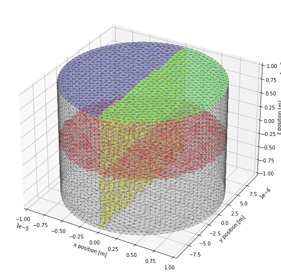
We use matplotlib Poly3DCollection to display collections of triangles. For convenience we define a small function that will plot the triangles with identical settings. The third parameter corresponds to the color of the triangles, it is a 4-tuple where each value is between 0 and 1. The first 3 represent respectively the amount of red, green and blue and the last one represents an alpha value controlling transparency. We plot the surface of the whole mesh in grey, patch1 in green, patch2 in blue, the diffusion boundary between comp1 and comp2 in red and the diffSurf surface along which we will record Species X concentrations in yellow. Note that matplotlib is not very well suited to plotting 3D data and projection issues may arise when the bounding boxes of Poly3DCollection overlap. To prevent this, we split the red and yellow surfaces in 2 pieces so that the overlap between their bounding boxes is minimal.

5.4. Simulation and data saving

Having defined our model and our geometry, we then create the simulation and specify which data should be saved.

rng = RNG('mt19937', 512, 2903)

sim = Simulation('Tetexact', mdl, mesh, rng)

rs = ResultSelector(sim)

XConcRand   = rs.TETS(randTets).X.Conc
YCountPatch = rs.TRIS(patchSurf).Y.Count
XCountSlice = rs.TETS(diffSlice).X.Count

Model checking:
No errors were found

Since we now use a tetrahedral mesh, we need to use a different solver. The 'Tetexact' solver builds on the 'Wmdirect' solver (we have used up until now) extended for diffusive fluxes between tetrahedral elements in a mesh. Each individual tetrahedron (triangle) behaves like a well-mixed compartment (patch) where reactions can take place. Diffusive flux between elements is represented by a series of first-order reactions with rate constants derived from the local geometry and the diffusion constant parameter. Thus, even though we only focus on diffusion here, this solver can be used to simulate full reaction-diffusion systems in complex geometries.

We want to save the concentration of X in the random tetrahedrons we selected. The corresponding ResultSelector path is rs.TETS(randTets).X.Conc. Instead of putting a compartment or patch name in second position, we use the TETS function and supply our list of random tetrahedrons as parameter. The resulting ResultSelector XConcRand has the same length as the randTets list. The following functions are available as a substitute for a geometrical location:

Syntax	Description	Length
TETS(lst)	Tetrahedrons in lst	len(lst)
TRIS(lst)	Triangles in lst	len(lst)
VERTS(lst)	Vertices in lst	len(lst)
TET(tet)	Tetrahedron tet	1
TET(x, y, z)	Tetrahedron at position x, y, z	1
TRI(tri)	Triangle tri	1
VERT(vert)	Vertex vert	1

XCountSlice and YCountPatch follow the same pattern. Note that the same functions apply to simulation paths, one could set the count of X in all tetrahedrons in list lst using:

sim.TETS(lst).X.Count = value

5.4.1. Metadata saving

The next chapter will introduce data recording to separate files that can then be loaded in a separate python process. In that case, information about the mesh will not necessarily be available when plotting the data, and we need to store it as metadata in the result selectors. For XConcRand for example, it will not be possible to know to which tetrahedron each column of the data corresponds to. Although we do not save the data to files in this current chapter, we will introduce how to save metadata in results selectors. By metadata we mean additional data that does not change with simulation time and that is specific to each recorded value in a result selector. This metadata is specified with the metaData property of the ResultSelectors. In the same way as we could provide custom labels in the previous chapter, we can associate arbitrary string keys with lists that have the same length as the ResultSelector. For XConcRand, we need to know what is the distance between each tetrahedron and the centeral tetrahedron in order to plot X concentrations as a function of the distance to the injection site. We thus add a metadata list with keyword 'distToCenter':

XConcRand.metaData['distToCenter'] = [np.linalg.norm(tet.center) for tet in randTets]

Since XCondRand was declared using the randTets list, we use the same list so that the distances are in the same order. np.linalg.norm() computes the \(\mathrm{L}^2\) norm of a numpy array; since we want to compute the distance between the tetrahedron center and the (0, 0, 0) point, we can directly feed tet.center to the norm function.

We then compute the distance to center for surface diffusion in the YCountPatch ResultSelector as well as the area of each triangle:

YCountPatch.metaData['distToCenter'] = [
    np.linalg.norm(tri.center[:2]) for tri in patchSurf
]
YCountPatch.metaData['triArea'] = [tri.Area for tri in patchSurf]

Here we restrict tri.center to the x and y coordinates with tri.center[:2] so that we can again feed it directly to the norm function.

Finally, for XCountSlice, we need to save the index of the triangle associated to each tetrahedron as well as the volume of each tetrahedron:

XCountSlice.metaData['surfTri'] = triInds
XCountSlice.metaData['tetVol'] = [tet.Vol for tet in diffSlice]

We then add the ResultSelectors to the simulation:

sim.toSave(XConcRand, timePoints=[ENDT])
sim.toSave(XCountSlice, YCountPatch, dt=0.01)

We want to save data every 0.01s for XCountSlice and YCountPatch but we only need to save XConcRand once, at the end of the simulation. To do so, we use the timePoints keyword argument instead of dt in the toSave function.

5.5. Running the simulations

We are now ready to run our simulations. This will look quite similar to our previous code for running well-mixed simulations, but this time we are injecting molecules into and recording data from individual tetrahedrons, not the whole compartment (though this is also possible). As initial conditions, we set the number of molecules in the central tetrahedron (or triangle) at time t = 0 to the number stored in variable NINJECT (or SNINJECT). By default all elements have their counts of all species set to zero.

During our geometry construction we already created our steps.geom.DiffBoundary object which will be included in the simulation, with the default behaviour to block diffusion between compartments comp1 and comp2 completely for all molecules. We now wish to allow diffusion of species ‘X’ through the boundary which we achieve by initializing the DiffusionActive property of the diffusion boundaries for species X to True. The same remark applies to the surface diffusion of species Y and the surface diffusion boundary between patch1 and patch2.

We now first run a series of NBRUNS runs in which both volume and surface diffusion are unaffected by the diffusion boundaries:

for r in range(NBRUNS):
    sim.newRun()
    sim.TET(centerTet).X.Count = NINJECT
    sim.TRI(topTri).Y.Count = SNINJECT
    sim.diffb.X.DiffusionActive = True
    sim.sdiffb.Y.DiffusionActive = True
    sim.run(ENDT)

We next want to activate the diffusion boundaries and prevent diffusion completely. To do so, we leave the DiffusionActive property of the diffusion boundaries to its default value which is False. Note that this property is defined in relation to a species. If we had another species X2 undergoing volume diffusion, we could block diffusion for X but not for X2 with:

sim.diffb.X.DiffusionActive = False
sim.diffb.X2.DiffusionActive = True

Let us run these simulations with:

for r in range(NBRUNS):
    sim.newRun()
    sim.TET(centerTet).X.Count = NINJECT
    sim.TRI(topTri).Y.Count = SNINJECT
    sim.run(ENDT)

Finally, the last batch of runs has active diffusion across the diffusion boundaries but the diffusion constant at which this diffusion occurs is 10 times smaller than the original value. We can do this by setting the Dcst property of the diffusion boundaries. As for DiffusionActive, this property is always defined in relation with a specific species:

for r in range(NBRUNS):
    sim.newRun()
    sim.TET(centerTet).X.Count = NINJECT
    sim.TRI(topTri).Y.Count = SNINJECT
    sim.diffb.X.Dcst = DCST / 10
    sim.sdiffb.Y.Dcst = SDCST / 10
    sim.run(ENDT)

Note that setting the Dcst property to a non-zero value automatically sets DiffusionActive to True.

5.6. Plotting the results

5.6.1. Simple scatter plots

So now we come to plotting our data. Now that we have spatial information the data we wish to plot is different to our previous well-mixed simulations where we were plotting the concentration in a well-mixed compartment. We will plot the mean concentration from individual tetrahedrons (or triangles) against their radial distance from origin.

We would first like to compare the spatial profile of the concentration of species X at the end of the simulation to the expected theoretical profile.

import matplotlib.pyplot as plt
from matplotlib.collections import PolyCollection
from matplotlib.colors import Normalize
from matplotlib import colormaps
import matplotlib.cm as cm
import numpy as np

plt.figure(figsize=(10, 7))

distances = XConcRand.metaData['distToCenter']
concentrs = np.mean(XConcRand.data[0:NBRUNS, -1, :], axis=0) * 1e6

plt.scatter(distances * 1e6, concentrs, s=10, label='Simulations')

def volDiffFunc(r, t):
    # Analytical value of C(r, t)
    Crt = NINJECT * np.exp(-(r**2) / (4 * DCST * t)) / (8 * (np.pi * DCST * t)**1.5)
    # Convert from number of molecules per m^3 to uM
    return Crt * (1e3 / 6.022e23)

rvals = np.linspace(0, max(distances), 100)
plt.plot(rvals * 1e6, [volDiffFunc(r, ENDT) for r in rvals], 'r', label='Theory')

plt.xlabel('Distance [μm]')
plt.ylabel('Concentration [μM]')
plt.title(f'Unbounded volume diffusion, time = {ENDT}s')
plt.legend()
plt.show()

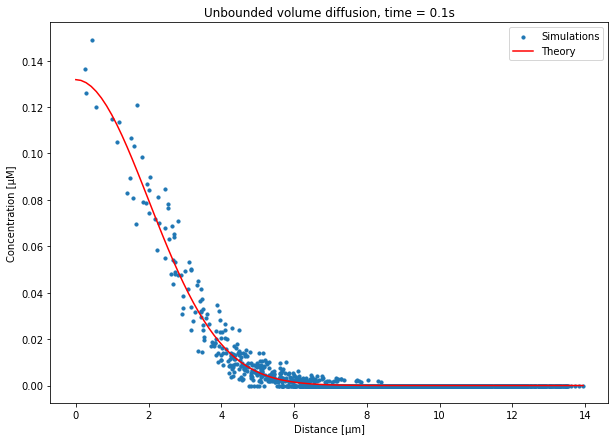
Since we do not have access to previously defined variables, we first need to reimport some packages and redeclare some of the parameters. The parameters are only needed in order to compute the analytical concentration profile. We then load the XConcRand ResultSelector, as we saw in the previous chapter. Distances from the center are retrieved using:

distances = XConcRand.metaData['distToCenter']

We then retrieve the concentration of species X at the end of the simulation in each tetrahedron and for each run with XConcRand.data[0:NBRUNS, -1, :], compute the average across runs, and convert the units to μM. Note that we retrict the runs to 0:NBRUNS since subsequent runs have different settings for the diffusion boundaries.

We then proceed to creating the same plot but for surface diffusion:

plt.figure(figsize=(10, 7))

distances  = YCountPatch.metaData['distToCenter']
counts     = np.mean(YCountPatch.data[0:NBRUNS, -1, :], axis=0)
countsPerA = counts / YCountPatch.metaData['triArea'] * 1e-12

plt.scatter(distances * 1e6, countsPerA, s=10, label='Simulations')

def surfDiffFunc(r, t):
    # Analytical value of C(r, t)
    Crt = SNINJECT * np.exp(-(r**2) / (4 * SDCST * t)) / (4 * np.pi * SDCST * t)
    # Convert from number per m^2 to number per um^2
    return Crt * 1e-12

rvals = np.linspace(0, max(distances), 100)
plt.plot(rvals * 1e6, [surfDiffFunc(r, ENDT) for r in rvals], 'r', label='Theory')

plt.xlabel('Distance [μm]')
plt.ylabel('Concentration [1/μm²]')
plt.title(f'Unbounded surface diffusion, time = {ENDT}s')
plt.legend()
plt.show()

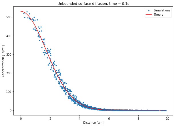
The main differences with the volume diffusion is that we saved the counts in each triangle and we thus need to compute a “surface concentration” (in \(\mathrm{\mu m}^{-2}\)) using the triangle areas we saved to metadata.

5.6.2. 2D spatial concentration profiles

Next, we turn to plotting a color coded 2D concentration profile of volume diffusion at different time points of the simulation. This is a bit more involved than the two previous plots and we thus need to define some helper functions:

def PlotProjectedSurface(fig, ax, triangles, values, proj, xlabel, ylabel, clabel):
    cmap = colormaps['viridis']
    maxVal = max(values)

    projTris = [[v @ proj.T for v in tri.verts] for tri in triangles]
    ax.add_collection(PolyCollection(
        projTris,
        facecolor=[cmap(v / maxVal) for v in values],
        edgecolors='black',
        linewidth=0.1
    ))

    fig.colorbar(
        cm.ScalarMappable(norm=Normalize(vmin=0, vmax=maxVal),cmap=cmap),
        ax=ax, label=clabel
    )

    minPoint = np.min(projTris, axis=(0, 1))
    maxPoint = np.max(projTris, axis=(0, 1))
    ax.set_xlim(minPoint[0], maxPoint[0])
    ax.set_ylim(minPoint[1], maxPoint[1])
    ax.set_xlabel(xlabel)
    ax.set_ylabel(ylabel)

Our first helper function will take a list of triangles, each associated to a numerical value, and will plot color-coded triangles in a 2D plot. Since the original triangles are in a 3D mesh, we also need to define a plane to which the data will be projected. We define this plane with the proj parameter, that should contain the unit x vector and the unit y vector of the desired plot in the 3D space. For each triangle, we then compute the projected positions of its vertices with:

projTris = [[v @ proj.T for v in tri.verts] for tri in triangles]

We then add all triangles to the plot and specify their color with the facecolor parameter. Since we directly plot triangles instead of using a dedicated matplotlib method, we need to explicitely specify the colorbar. Finaly, we determine the bounding box of the projected triangles and restrict the plot to it.

Next, we define another helper function that will take one of our XCountSlice... ResultSelectors and plot the 2D concentration profile at different time points:

def PlotSliceConc(results, runStart, runEnd, mesh, tinds, proj, xlabel, ylabel, clabel):
    fig = plt.figure(figsize=(6, 15))

    for i, tind in enumerate(tinds):
        ax = fig.add_subplot(len(tinds), 1, i+1)
        ax.set_aspect("equal")

        triangles = TriList(results.metaData['surfTri'][::2], mesh=mesh)

        mean = np.mean(results.data[runStart:runEnd, tind, :], axis=0)
        tetCounts = np.reshape(mean, (len(mean) // 2, 2))
        tetVols = np.reshape(results.metaData['tetVol'], (len(mean) // 2, 2))
        values = np.sum(tetCounts, axis=1) / 6.02214076e23 / np.sum(tetVols, axis=1) * 1e3

        PlotProjectedSurface(fig, ax, triangles, values, proj, xlabel, ylabel, clabel)

        ax.set_title(f'time = {results.time[0][tind]}s')
        if i < len(tinds) - 1:
            ax.set_xlabel(None)
            ax.set_xticklabels([])

    plt.show()

Since we only saved the indexes of the triangles, this helper function will need the mesh as a parameter. Let us remind ourselves that the XCountSlice ResultSelector saved the counts of species X in the two tetrahedrons neighbors of each triangle. The data is thus somehow grouped by pairs of values and we need a way to compute, for each triangle, the average concentration of X in its 2 tetrahedron neighbors. We first create the list of triangles with:

triangles = TriList(results.metaData['surfTri'][::2], mesh=mesh)

saver.metaData['surfTri'] outputs a vector whose length is twice the number of triangles, and since the tetrahedrons are ordered by associated triangles, we know that the triangle indexes at 2k and 2k+1 are identical. We thus only select the indexes at 2k with [::2].

We then compute the average counts in tetrahedrons across all runs and reshape the data to group values that are associated with the same triangle with:

tetCounts = np.reshape(mean, (len(mean) // 2, 2))

tetCounts now contains, for each triangle, the counts of X of its 2 tetrahedron neighbors. We then reshape the tetrahedron volumes in the same way and compute the concentration associated with each triangle with:

values = np.sum(tetCounts, axis=1) / 6.02214076e23 / np.sum(tetVols, axis=1) * 1e3

We use the numpy sum function with axis=1 to compute, for each triangle, the sum of counts and the sum of volumes in each tetrahedron neighbor. We divide the counts by Avogadro’s constant and by the volumes to get a concentration that we express in μM. We then call our previously defined helper function to plot the color-coded triangles. We can now finally plot the results! We first look at unconstrained volume diffusion by loading the XCountSlice ResultSelector. We select 3 time points between t = 0.01 and t = TEND and declare the axes to wich we want to project the data:

tinds = np.linspace(1, len(XCountSlice.time[0]) - 1, 3).astype(int)
proj = np.array([
    [0, 1e6, 0],
    [0, 0, 1e6]
])
xlbl = 'y position [μm]'
ylbl = 'z position [μm]'
clbl = 'X Concentration [μM]'

PlotSliceConc(XCountSlice, 0, NBRUNS, mesh, tinds, proj, xlbl, ylbl, clbl)

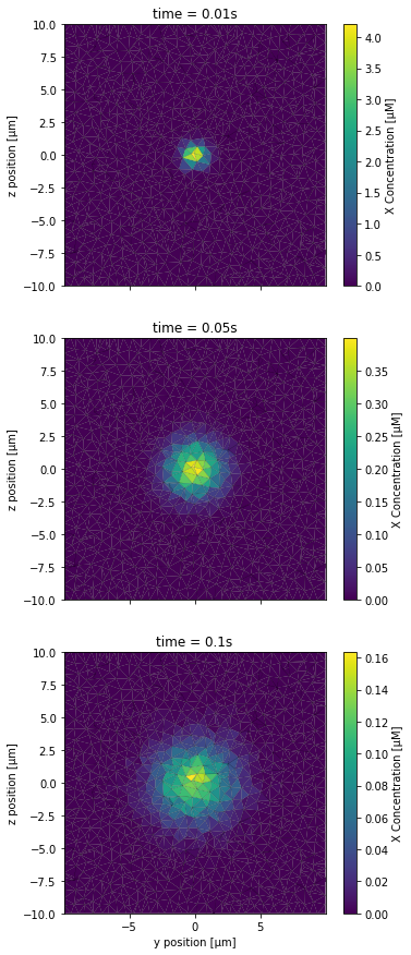
The x axis of the plot corresponds to the y axis of the full 3D space and the y axis of the plot to the z axis of the 3D space; we scale all distances to μm. Note that each subplot has its own color scale because the maximum concentrations at t = 0.01s are much higher than for the other time points and a single color scale would prevent seeing the concentration gradients on the 3 other subplots.

We next create the same plots but for the scenario in which we prevented diffusion across the z = 0 plane:

PlotSliceConc(XCountSlice, NBRUNS, 2*NBRUNS, mesh, tinds, proj, xlbl, ylbl, clbl)

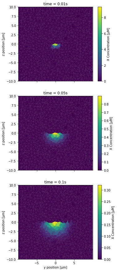
As expected, one half of the slice did not receive any species X. Finally, we take a look at the scenario in which the diffusion boundary restricted diffusion to a tenth of its original value:

PlotSliceConc(XCountSlice, 2*NBRUNS, 3*NBRUNS, mesh, tinds, proj, xlbl, ylbl, clbl)

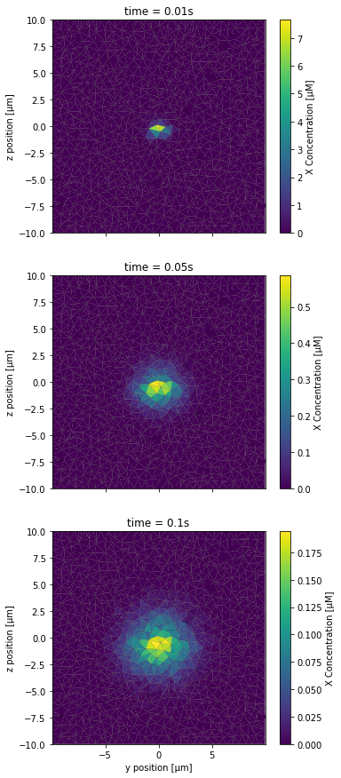
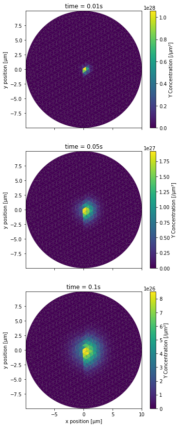
We now would like to make the same types of plots but for the surface diffusion boundary data. We first need to define a helper function that is similar to PlotSliceConc but simpler since the data we recorded is directly associted to each triangles of the top surface of the cylinder. We thus define PlotPatchConc as:

def PlotPatchConc(results, runStart, runEnd, mesh, tinds, proj, xlabel, ylabel, clabel):
    fig = plt.figure(figsize=(6, 15))

    for i, tind in enumerate(tinds):
        ax = fig.add_subplot(len(tinds), 1, i+1)
        ax.set_aspect("equal")

        triangles = TriList([ind for ind in results.metaData['loc_id']], mesh=mesh)
        values = np.mean(results.data[runStart:runEnd, tind, :], axis=0)
        values /= results.metaData['triArea'] * 1e-12

        PlotProjectedSurface(fig, ax, triangles, values, proj, xlabel, ylabel, clabel)

        ax.set_title(f'time = {results.time[0][tind]}s')
        if i < len(tinds) - 1:
            ax.set_xlabel(None)
            ax.set_xticklabels([])

    plt.show()

For each time point, we first create the list of triangles. Note that this time we did not explicitely save the index of each triangles as metadata when we declared our ResultSelector, instead we use automatically declared metadata 'loc_id' that contains the identifiers of the geometrical location for which the data is saved. If this location is a patch or a compartment, this will contain its name, if it is a tetrahedron or a triangle, it will contain its index in the mesh. The following metadata are automatically declared for all ResultSelectors:

Metadata key	Description	Value
'loc_type'	Geometrical location type	'Tet' for tetrahedrons, 'Tri' for triangles, 'Patch' for patches, etc.
'loc_id'	Identifier of geometrical location	Name for patches or compartment, mesh index for tetrahedrons or triangles
'parent_loc_type'	Parent geometrical location type	Only defined for tetrahedrons and triangles, type of the compartment or patch to which the element is associated, if any
'parent_loc_id'	Parent identifier	Only defined for tetrahedrons and triangles, name of the compartment or patch to which the element is associated, if any
'obj_type'	Object type	'Species' for species, 'Reaction' for reactions, etc.
'obj_id'	Object identifier	Name of species, reaction, etc.

Note that we have to specify the mesh explicitely when creating the TriList since we are not in a with mesh: block. The values associated to each triangle are then computed and scaled to be expressed in \(\mathrm{\mu m}^{-2}\). The triangles are plotted using the first helper function we defined. All that is left to do now is to specify the referential in which the triangles should be projected and to load the data. We will first do so for the unconstrained surface diffusion scenario:

proj = np.array([
    [1e6, 0, 0],
    [0, 1e6, 0]
])
xlbl = 'x position [μm]'
ylbl = 'y position [μm]'
clbl = 'Y Concentration [/μm²]'

PlotPatchConc(YCountPatch, 0, NBRUNS, mesh, tinds, proj, xlbl, ylbl, clbl)

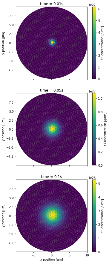
This time we wanted to have a top down view of the top surface of the cylinder. Both the x and y axes of the plot thus correspond to the x and y axes of the 3D space, with distances being scaled to μm. We then create the same plots for the 2 remaining scenarios. First for the completely blocking diffusion boundary scenario:

PlotPatchConc(YCountPatch, NBRUNS, 2*NBRUNS, mesh, tinds, proj, xlbl, ylbl, clbl)

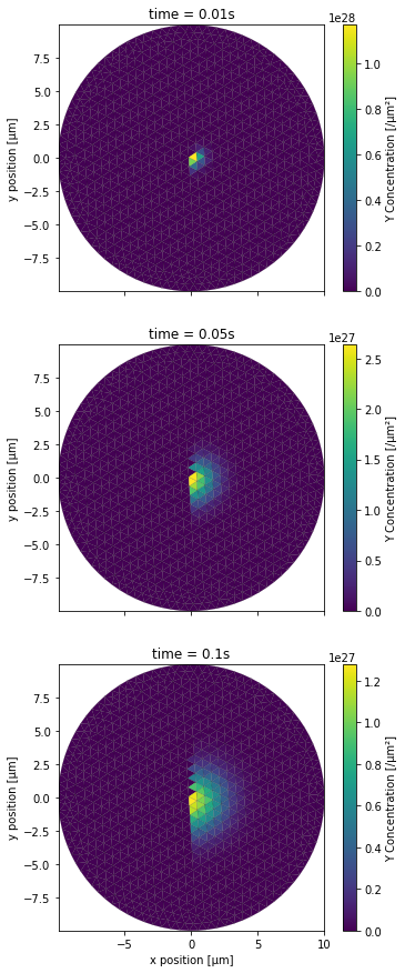
Then for the partially blocking one:

PlotPatchConc(YCountPatch, 2*NBRUNS, 3*NBRUNS, mesh, tinds, proj, xlbl, ylbl, clbl)

5.6.3. Directional diffusion

In this chapter we saw how to change a diffusion constant with the Dcst property. For example, we changed the diffusion constant of the diffusion boundary diffb with sim.diffb.X.Dcst = DCST / 10. diffb sits between comp1 and comp2 and the diffusion constant applies to both diffusion from comp1 to comp2 and diffusion from comp2 to comp1. STEPS also allows to set the diffusion constant for a specific direction with e.g.:

sim.diffdb(direc=comp2).SA.Dcst = DCST / 2
sim.diffdb(direc=comp1).SA.Dcst = 0

With this code, we set the diffusion of SA from comp1 to comp2 to be DCST / 2 and we suppress diffusion of SA from comp2 to comp1. Note that we use parentheses to further specify sdiffdb in the simulation path.

The same thing can be done at the level of tetrahedrons:

sim.TET(tet1).volDiff(direc=tet2).D = DCST / 10

Assuming that we named a volume diffusion rule volDiff, the above code sets the diffusion constant from tet1 to tet2 (which need to be neighboring tetrahedrons in the same compartment). Note that we do not need to specify the species to which this applies since it is already specified in the volDiff diffusion rule.

Similarly, for surface diffusion rules and triangles:

sim.TRI(tri1).surfDiff(direc=tri2).D = SDCST / 10

Like for tetrahedrons, tri1 and tri2 need to be neighboring triangles in the same patch.