12. Distributed mesh simulations
Topics: Distributed mesh solver, Local mesh elements, distributed data saving.
Althouth the 'TetOpSplit' solver runs simulations in parallel, the mesh is still fully loaded in each of the MPI processes. This can become a limiting factor when larger meshes are used. Since STEPS 4.0, a new solver, 'DistTetOpSplit' was added to tackle this issue. This solver loads the mesh in a distributed way, meaning that each MPI process only loads the part of the mesh that it will simulate.
For more details about the performace of the 'DistTetOpSplit' distributed mesh solver, please check the following paper:
Weiliang Chen, Tristan Carel, Omar Awile, Nicola Cantarutti, Giacomo Castiglioni, Alessandro Cattabiani, Baudouin Del Marmol, Iain Hepburn, James G King, Christos Kotsalos, Pramod Kumbhar, Jules Lallouette, Samuel Melchior, Felix Schürmann, Erik De Schutter (2022). STEPS 4.0: Fast and memory-efficient molecular simulations of neurons at the nanoscale. Front. Neuroinform. Volume 16. https://doi.org/10.3389/fninf.2022.883742.
12.1. Converting parallel simulations to distributed
Changing from the 'TetOpSplit' parallel solver to the 'DistTetOpSplit' distributed solver requires a few extra changes to STEPS python scripts. To show these changes, we will use a slightly modified version of the stochastic calcium burst model introduced previously. We will not go through the entire script but we will focus instead on the parts that are relevant to distributed simulations.
The script that we will use in this chapter can be downloaded here:
import steps.interface

from steps.geom import *
from steps.model import *
from steps.rng import *
from steps.saving import *
from steps.sim import *
from steps.utils import *

import numpy as np

# # # # # # # # # # # # # # # # # # # # # # # # # # # # # # # # # # # # # # # #

###########################################################
# Simulation Parameters
###########################################################

ENDT = 0.06

DT =  2.0e-5

EF_DT = 5.0e-6

SEED = 1234

###########################################################
# Model Parameters
###########################################################

TEMPERATURE = 34.0 + 273.15
Q10 = 3

FARADAY = 96485.3365     # C/mol
R = 8.3144621            # J/mol K
AVOGADRO = 6.02214129e23 # /mol

Qt = Q10 ** ((TEMPERATURE - (23 + 273.15)) / 10)
Qt_mslo = Q10 ** ((TEMPERATURE - (25 + 273.15))/10)

#######################################
# Membrane Parameters
#######################################

init_pot = Parameter(-60, 'mV', Description='Initial membrane potential')
Ra = Parameter(235.7*1.0e-2, 'ohm m', Description='Bulk resistivity')
Cm = 0.64e-2
memb_capac_proximal = Parameter(1.2*Cm, 'F m^-2', Description='Smooth membrane capacitance')
memb_capac_spiny = Parameter(5.3*Cm, 'F m^-2', Description='Spiny membrane capacitance')

#######################################
# CaP channels parameters
#######################################

CaP_P = Parameter(2.5e-2, 'um^3 s^-1', Description='CaP single channel permeability')
CaP_ro = Parameter(38, 'um^-2', Description='CaP channels density')

# Reaction rates

vhalfm = -29.458 # mV
cvm = 8.429      # mV

def minf_cap(mV):
    vhalfm = -29.458
    cvm = 8.429
    return 1 / (1 + np.exp(-(mV - vhalfm) / cvm))

def tau_cap(mV):
    if mV >= -40:
        return 0.2702 + 1.1622 * np.exp(-(mV + 26.798) ** 2 / 164.19)
    else:
        return 0.6923 * np.exp(mV / 1089.372)

alpha_cap = VDepRate.Create(
    lambda V: (minf_cap(V * 1e3) / tau_cap(V * 1e3)) * Qt * 1e3
)
beta_cap = VDepRate.Create(
    lambda V: (1 - minf_cap(V * 1e3)) / tau_cap(V * 1e3) * Qt * 1e3
)

# Initial conditions
CaP_p = [0.92402, 0.073988, 0.0019748, 1.7569e-05]

#######################################
# CaT channels parameters
#######################################

CaT_P = Parameter(1.65e-2, 'um^3 s^-1', Description='CaT single channel permeability')
CaT_ro = Parameter(1.9636, 'um^-2', Description='CaT channels density')

# Reaction rates

def minf_cat(mV):
    vhalfm = -52
    cvm = -5
    return 1 / (1 + np.exp((mV - vhalfm) / cvm))

def taum_cat(mV):
    if mV > -90:
        return 1 + 1 / (np.exp((mV + 40) / 9) + np.exp(-(mV + 102) / 18))
    else:
        return 1

def hinf_cat(mV):
    vhalfh = -72
    cvh = 7
    return 1 / (1 + np.exp((mV - vhalfh) / cvh))

def tauh_cat(mV):
    return (15 + 1 / (np.exp((mV + 32) / 7)))

alpham_cat = VDepRate.Create(lambda V: minf_cat(V * 1e3) / taum_cat(V * 1e3) * 1e3)
betam_cat = VDepRate.Create(lambda V: (1 - minf_cat(V * 1e3)) / taum_cat(V * 1e3) * 1e3)

alphah_cat = VDepRate.Create(lambda V: hinf_cat(V * 1e3) / tauh_cat(V * 1e3) * 1e3)
betah_cat = VDepRate.Create(lambda V: (1 - hinf_cat(V * 1e3)) / tauh_cat(V * 1e3) * 1e3)

# Initial conditions
CaT_p = [
    [0.58661, 0.23687, 0.023912],   # h0
    [0.10564, 0.042658, 0.0043063], # h1
]

#######################################
# BK channels parameters
#######################################

BK_G = Parameter(210, 'pS', Description='BK single channel conductance')
BK_ro = Parameter(1.5 * 2.0238, 'um^-2', Description='BK channels density')
BK_rev = Parameter(-77, 'mV', Description='BK channel reversal potential')

# Reaction rates

#Units (1)
Qo = 0.73
Qc = -0.67

#Units (/s)
pf0 = 2.39
pf1 = 5.4918
pf2 = 24.6205
pf3 = 142.4546
pf4 = 211.0220

pb0 = 3936
pb1 = 687.3251
pb2 = 234.5875
pb3 = 103.2204
pb4 = 11.6581

#Units(/M)
k1 = 1.0e6

#Units(/s)
onoffrate = 1.0e3

L0 = 1806

#Units (M)
Kc = 8.63e-6
Ko = 0.6563e-6

BK_f = k1*onoffrate*Qt_mslo
BKo_b = Ko*k1*onoffrate*Qt_mslo
BKc_b = Kc*k1*onoffrate*Qt_mslo

BK_f0 = VDepRate.Create(
    lambda V: pf0 * Qt_mslo * (np.exp((Qo * FARADAY * V) / (R * TEMPERATURE)))
)
BK_f1 = VDepRate.Create(
    lambda V: pf1 * Qt_mslo * (np.exp((Qo * FARADAY * V) / (R * TEMPERATURE)))
)
BK_f2 = VDepRate.Create(
    lambda V: pf2 * Qt_mslo * (np.exp((Qo * FARADAY * V) / (R * TEMPERATURE)))
)
BK_f3 = VDepRate.Create(
    lambda V: pf3 * Qt_mslo * (np.exp((Qo * FARADAY * V) / (R * TEMPERATURE)))
)
BK_f4 = VDepRate.Create(
    lambda V: pf4 * Qt_mslo * (np.exp((Qo * FARADAY * V) / (R * TEMPERATURE)))
)
BK_oc_f = [BK_f0, BK_f1, BK_f2, BK_f3, BK_f4]

BK_b0 = VDepRate.Create(
    lambda V: pb0 * Qt_mslo * (np.exp((Qc * FARADAY * V) / (R * TEMPERATURE)))
)
BK_b1 = VDepRate.Create(
    lambda V: pb1 * Qt_mslo * (np.exp((Qc * FARADAY * V) / (R * TEMPERATURE)))
)
BK_b2 = VDepRate.Create(
    lambda V: pb2 * Qt_mslo * (np.exp((Qc * FARADAY * V) / (R * TEMPERATURE)))
)
BK_b3 = VDepRate.Create(
    lambda V: pb3 * Qt_mslo * (np.exp((Qc * FARADAY * V) / (R * TEMPERATURE)))
)
BK_b4 = VDepRate.Create(
    lambda V: pb4 * Qt_mslo * (np.exp((Qc * FARADAY * V) / (R * TEMPERATURE)))
)
BK_oc_b = [BK_b0, BK_b1, BK_b2, BK_b3, BK_b4]

# Initial conditions
BK_p = [
    [0.99997,    4.3619e-07, 4.1713e-09, 4.4449e-11, 6.3132e-14],
    [2.5202e-05, 1.1765e-06, 6.6148e-08, 2.4392e-09, 4.0981e-11],
]

#######################################
# SK channels parameters
#######################################

SK_G = Parameter(10, 'pS', Description='SK single channel conductance')
SK_ro = Parameter(0.31, 'um^-2', Description='SK channels density')
SK_rev = Parameter(-77, 'mV', Description='SK channel reversal potential')

# Reaction rates

#Units (/s)
invc1 = 80
invc2 = 80
invc3 = 200

invo1 = 1000
invo2 = 100

diro1 = 160
diro2 = 1200

#Units ( /s M)

dirc2 = 200e6
dirc3 = 160e6
dirc4 = 80e6

invc1_t = invc1*Qt
invc2_t = invc2*Qt
invc3_t = invc3*Qt

invo1_t = invo1*Qt
invo2_t = invo2*Qt

diro1_t = diro1*Qt
diro2_t = diro2*Qt

dirc2_t = dirc2*Qt/3.0
dirc3_t = dirc3*Qt/3.0
dirc4_t = dirc4*Qt/3.0

# Intital conditions
SK_C1_p= 0.96256
SK_C2_p= 0.036096
SK_C3_p= 0.0010829
SK_C4_p= 6.4973e-06

SK_O1_p= 0.00017326
SK_O2_p= 7.7967e-05

#######################################
# AMPA channels parameters
#######################################

AMPA_G = Parameter(7, 'pS', Description="AMPA channel conductance")
AMPA_Ro = Parameter(20, 'um^-2', Description="AMPA channek density")
AMPA_rev = Parameter(0, 'mV', Description="AMPA channel reversal potential")

#Units (/s M)

rb = 13e6

#Units (/s)

ru1 = 0.0059e3
ru2 = 86e3
ro = 2.7e3
rc = 0.2e3
rd = 0.9e3
rr = 0.064e3

# Glutamate transient

# Units (s)

glut_start = 5e-3

# Units (M), Reference (Rudolph et al. 2011)
def Glut(t):
    if t >= 0:
        return 12e-3 * (0.86 * np.exp(-t / 0.4e-3) + 0.14 * np.exp(-t / 4.2e-3))
    else:
        return 0

#######################################
# Leak channels parameters
#######################################

L_G = Parameter(0.4, 'pS', Description='Leak single channel conductance')
L_ro_proximal = Parameter(0.25, 'um^-2', Description='Proximal leak channels density')
L_ro_spiny = Parameter(1, 'um^-2', Description='Proximal leak channels density')
L_rev = Parameter(-61, 'mV', Description='Leak channel reversal potential')

#######################################
# Ca pump channels parameters
#######################################

P_ro = Parameter(6.022141, 'um^-2', Description='Ca2+ pump density')

# Reaction rates

P_f = 3e9
P_b = 1.75e4
P_k = 7.255e4

#######################################
# Calcium buffering parameters
#######################################

# Ca concentrations

Ca_oconc = 2e-3
Ca_iconc = 45e-9

# Mg concentrations

Mg_conc = 590e-6

# Buffer concentrations

iCBsf_conc = 27.704e-6
iCBCaf_conc = 2.6372e-6
iCBsCa_conc= 1.5148e-6
iCBCaCa_conc= 0.14420e-6

CBsf_conc= 110.82e-6
CBCaf_conc= 10.549e-6
CBsCa_conc= 6.0595e-6
CBCaCa_conc= 0.57682e-6

PV_conc= 3.2066e-6
PVCa_conc= 16.252e-6
PVMg_conc= 60.541e-6

# Diffusion constants

DCST = 0.223e-9 # Ca
DCB = 0.028e-9  # Calbindin (CB)
DPV = 0.043e-9  # Parvalbumin (PV)

# Reaction rates

CBf_f_kcst = 4.35e7
CBf_b_kcst = 35.8

CBs_f_kcst = 0.55e7
CBs_b_kcst = 2.6

PVca_f = 10.7e7
PVca_b = 0.95

PVmg_f_kcst = 0.8e6
PVmg_b_kcst = 25

###########################################################
# Mesh Parameters
###########################################################

mesh_file = '../meshes/caburst_dist/split_256/CNG_segmented_2_split_256'

# # # # # # # # # # # # # # # # # # # # # # # # # # # # # # # # # # # # # # # #

###########################################################
# Biochemical model
###########################################################

mdl = Model()
with mdl:
    # Species
    Pump, CaPump, PV, PVMg, PVCa, Mg = Species.Create()
    Ca = Species.Create(valence=2)

    # Calbindin
    CBs, CBf, CBsCa, CBfCa, CBmob, CBimmob = SubUnitState.Create()
    CBsSU, CBfSU, CBmobSU = SubUnit.Create(
        [CBs, CBsCa], [CBf, CBfCa], [CBmob, CBimmob]
    )
    CB = Complex.Create([CBsSU, CBfSU, CBmobSU], statesAsSpecies=True)

    # Channels
    CaPc, CaPo = SubUnitState.Create()
    CaP_SU = SubUnit.Create([CaPc, CaPo])
    CaPchan = Channel.Create([CaP_SU, CaP_SU, CaP_SU])

    BK, BKCa, BKopen, BKclose = SubUnitState.Create()
    BKCaSU = SubUnit.Create([BK, BKCa])
    BKocSU = SubUnit.Create([BKopen, BKclose])
    BKchan = Channel.Create([BKCaSU, BKCaSU, BKCaSU, BKCaSU, BKocSU])

    SK_C1, SK_C2, SK_C3, SK_C4, SK_O1, SK_O2 = SubUnitState.Create()
    SKchan = Channel.Create([SK_C1, SK_C2, SK_C3, SK_C4, SK_O1, SK_O2])

    AMPA_C, AMPA_C1, AMPA_C2, AMPA_D1, AMPA_D2, AMPA_O = SubUnitState.Create()
    AMPA = Channel.Create([AMPA_C, AMPA_C1, AMPA_C2, AMPA_D1, AMPA_D2, AMPA_O])

    Leak = SubUnitState.Create()
    L = Channel.Create([Leak])

    r = ReactionManager()

    vsys = VolumeSystem.Create()
    with vsys:
        # PVCa
        PV + Ca <r[1]> PVCa
        r[1].K = PVca_f, PVca_b

        # PVMg
        PV + Mg <r[1]> PVMg
        r[1].K = PVmg_f_kcst, PVmg_b_kcst

        with CB[...]:
            # Fast binding
            CBf + Ca <r[1]> CBfCa
            r[1].K = CBf_f_kcst, CBf_b_kcst

            # Slow binding
            CBs + Ca <r[1]> CBsCa
            r[1].K = CBs_f_kcst, CBs_b_kcst

        diff_Ca   = Diffusion.Create(Ca, DCST)
        diff_CB   = Diffusion.Create(CB[:, :, CBmob], DCB)
        diff_PV   = Diffusion.Create(PV, DPV)
        diff_PVCa = Diffusion.Create(PVCa, DPV)
        diff_PVMg = Diffusion.Create(PVMg, DPV)

    ssys = SurfaceSystem.Create()
    with ssys:
        # Ca Pump
        Pump.s + Ca.i <r[1]> CaPump.s >r[2]> Pump.s
        r[1].K = P_f, P_b
        r[2].K = P_k

        # CaP channel
        with CaPchan[...]:
            CaPc.s <r[1]> CaPo.s
            r[1].K = VDepRate(alpha_cap), VDepRate(beta_cap)
        OC_CaP = GHKCurr.Create(
            CaPchan[CaPo, CaPo, CaPo], Ca, CaP_P,
            computeflux=True, virtual_oconc=Ca_oconc
        )

        # BK channel
        with BKchan[..., BKclose]:
            BK.s + Ca.i <r[1]> BKCa.s
            r[1].K = BK_f, BKc_b

        with BKchan[..., BKopen]:
            BK.s + Ca.i <r[1]> BKCa.s
            r[1].K = BK_f, BKo_b

        with BKchan[...]:
            BKclose.s <r[1]> BKopen.s
            r[1].K = (
                CompDepRate(lambda s: BK_oc_f[s.Count(BKCa)], [BKchan]),
                CompDepRate(lambda s: BK_oc_b[s.Count(BKCa)], [BKchan])
            )
        OC_BK = OhmicCurr.Create(BKchan[..., BKopen], BK_G, BK_rev)

        # SK channel
        with SKchan[...]:
            ((SK_C1.s + Ca.i <r[1]> SK_C2.s)\
                      + Ca.i <r[2]> SK_C3.s)\
                      + Ca.i <r[3]> SK_C4.s
            r[1].K = dirc2_t, invc1_t
            r[2].K = dirc3_t, invc2_t
            r[3].K = dirc4_t, invc3_t

            SK_C3.s <r[1]> SK_O1.s
            SK_C4.s <r[2]> SK_O2.s
            r[1].K = diro1_t, invo1_t
            r[2].K = diro2_t, invo2_t
        OC_SK = OhmicCurr.Create(SKchan[SK_O1|SK_O2], SK_G, SK_rev)

        # AMPA channel
        with AMPA[...]:
            AMPA_C.s <r['A1']> AMPA_C1.s <r['A2']> AMPA_C2.s <r[3]> AMPA_O.s
            r['A1'].K = 0, ru1
            r['A2'].K = 0, ru2
            r[3].K = ro, rc

            AMPA_C1.s <r[1]> AMPA_D1.s
            AMPA_C2.s <r[2]> AMPA_D2.s
            r[1].K = rd, rr
            r[2].K = rd, rr
        OC_AMPAR1 = OhmicCurr.Create(AMPA[AMPA_O], AMPA_G, AMPA_rev)

        # Leak current channel
        OC_L = OhmicCurr.Create(L[Leak], L_G, L_rev)

###########################################################
# Mesh and compartmentalization
###########################################################

mesh = DistMesh(mesh_file, 1e-6)

with mesh.asLocal(owned=False):
    cyto = Compartment.Create(mesh.tets, vsys)
    cyto.Conductivity = 1 / Ra

    smoothTets = mesh.tetGroups['smooth']
    spinyTets = mesh.tetGroups['spiny']

    smooth = Patch.Create(smoothTets.surface & mesh.surface, cyto, None, ssys)
    spiny = Patch.Create(spinyTets.surface & mesh.surface, cyto, None, ssys)

    memb_smooth = Membrane.Create([smooth], capacitance=memb_capac_proximal)
    memb_spiny = Membrane.Create([spiny], capacitance=memb_capac_spiny)

###########################################################
# Simulation
###########################################################

rng = RNG('mt19937', 512, SEED)

sim = Simulation(
    'DistTetOpSplit', mdl, mesh, rng,
    searchMethod=NextEventSearchMethod.GIBSON_BRUCK
)

rs = ResultSelector(sim)

with mesh.asLocal():
    Pots = rs.VERTS(mesh.surface.verts).V
    CaConc = rs.TETS().Ca.Conc
    CaConc.metaData['Vols'] = [tet.Vol for tet in mesh.tets]
    Currents = rs.TRIS(mesh.surface).OC_CaP.I

sim.toSave(Pots, CaConc, Currents, dt=DT)

with XDMFHandler('DistCaburst') as hdf:
    sim.toDB(hdf, 'CaBurstSim')

    sim.newRun()

    # Set temperature for ghk reactions
    sim.Temp = TEMPERATURE + 273.15

    # Setting initial conditions
    simPatches = [sim.smooth, sim.spiny]
    smoothArea = Parameter(smooth.Area, 'm^2')
    spinyArea = Parameter(spiny.Area, 'm^2')
    for patch, area in zip(simPatches, [smoothArea, spinyArea]):
        patch.Pump.Count = round(P_ro * area)

        for s in CaPchan[...]:
            patch.LIST(s).Count = round(CaP_ro*area*CaP_p[s.Count(CaPo)])

        for s in BKchan[...]:
            isOpen, nbCa = s.Count(BKopen), s.Count(BKCa)
            patch.LIST(s).Count = round(BK_ro*area*BK_p[isOpen][nbCa])

        patch.SKchan[SK_C1].Count = round(SK_ro*area*SK_C1_p)
        patch.SKchan[SK_C2].Count = round(SK_ro*area*SK_C2_p)
        patch.SKchan[SK_C3].Count = round(SK_ro*area*SK_C3_p)
        patch.SKchan[SK_C4].Count = round(SK_ro*area*SK_C4_p)
        patch.SKchan[SK_O1].Count = round(SK_ro*area*SK_O1_p)
        patch.SKchan[SK_O2].Count = round(SK_ro*area*SK_O2_p)

    sim.spiny.L[Leak].Count = round(L_ro_spiny * spinyArea)
    sim.smooth.L[Leak].Count = round(L_ro_proximal * smoothArea)

    sim.smooth.AMPA[AMPA_C].Count = round(AMPA_Ro * smoothArea)

    sim.cyto.Ca.Conc = Ca_iconc
    sim.cyto.Mg.Conc = Mg_conc

    sim.cyto.CB[CBs,   CBf,   CBimmob].Conc = iCBsf_conc
    sim.cyto.CB[CBsCa, CBf,   CBimmob].Conc = iCBCaf_conc
    sim.cyto.CB[CBs,   CBfCa, CBimmob].Conc = iCBsCa_conc
    sim.cyto.CB[CBsCa, CBfCa, CBimmob].Conc = iCBCaCa_conc

    sim.cyto.CB[CBs,   CBf,   CBmob].Conc = CBsf_conc
    sim.cyto.CB[CBsCa, CBf,   CBmob].Conc = CBCaf_conc
    sim.cyto.CB[CBs,   CBfCa, CBmob].Conc = CBsCa_conc
    sim.cyto.CB[CBsCa, CBfCa, CBmob].Conc = CBCaCa_conc

    sim.cyto.PV.Conc = PV_conc
    sim.cyto.PVCa.Conc = PVCa_conc
    sim.cyto.PVMg.Conc = PVMg_conc

    sim.EfieldDT = EF_DT

    sim.ALL(Membrane).Potential = init_pot

    for t in np.arange(0, ENDT, DT):
        if MPI.rank == 0:
            print(f'Run timestep {t}')
        # Update AMPA receptors reaction rate
        sim.smooth.A1['fwd'].K = rb * Glut(t - glut_start)
        sim.smooth.A2['fwd'].K = rb * Glut(t - glut_start)

        sim.run(t)
The biochemical model declaration does not involve anything specific to the distributed mesh solver and is thus identical for parallel or even serial simulations. In this chapter, we will mainly focus on the differences related to geometry declaration.
12.2. Mesh partionioning and loading
In this chapter, we will use the following reconstructed mesh of a Purkinje cell dendritic tree:
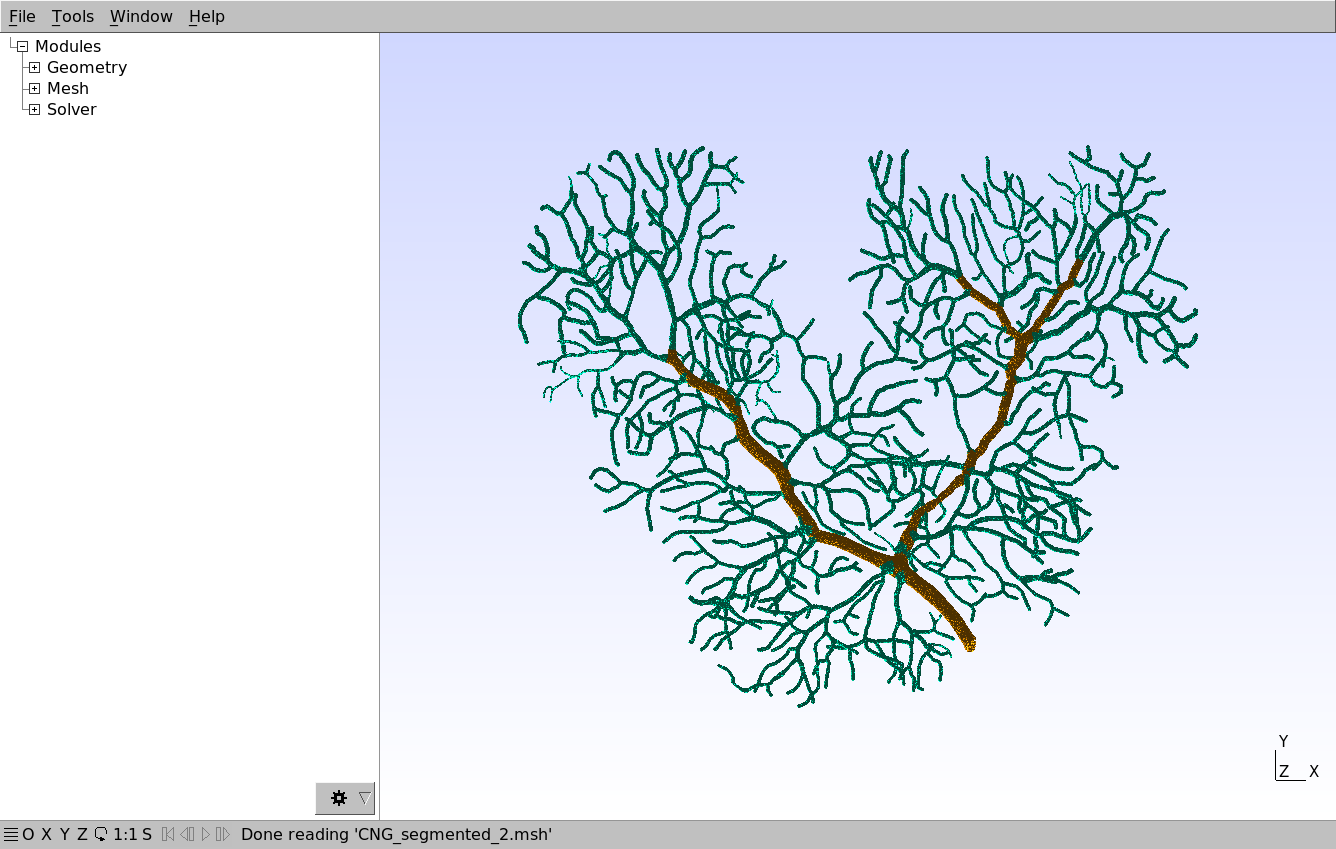
The mesh can be downloaded here and visualized with Gmsh. Note that the mesh tetrahedrons are classified and annotated into two components, representing smooth dendrite (orange) and spiny dendrite (green). These annotations will then be used in STEPS for creating corresponding patches.
Distributed meshes are created in the python script with Distmesh, a different class from the one that was used for parallel simulations (TetMesh). In contrast to TetMesh, that could load meshes from a variety of file formats, distributed meshes can only be created from meshes saved to the Gmsh format. However, while TetMeshes required an additional partitioning step in the python script, DistMesh can
automatically be partitioned upon mesh creation:
mesh = DistMesh('path/to/mesh_file.msh, scale=1e-6)
The above line loads and distributes the mesh. Like for TetMesh, it also takes a scale parameter to rescale the dimensions to meters, if needed.
Although the automatic partitioning is convenient, it can often lead to sub-optimal partitions in which spatially close but disconnected parts of the mesh are grouped in the same partition. In addition, the mesh has to be fully loaded by one MPI rank before being distributed, which can be an issue in cases where the mesh is too big to fully fit in memory. As we saw in the parallel simulations chapter, it is usually better to pre-partition meshes with dedicated partitioning software like Metis.
In this chapter, we will thus pre-partition the mesh from the Gmsh software but save each partition to a separate file, so that, when loaded into STEPS, each MPI rank will only load its part of the mesh in memory.
Once the mesh is loaded in Gmsh, it can be partitioned with Modules \(\rightarrow\) Mesh \(\rightarrow\) Partition, which opens the following dialog:
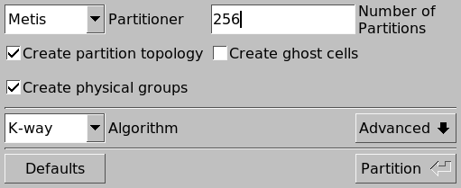
We will split it into 256 partitions using Metis. After the partitioning is complete, we can see the partitions that METIS created:
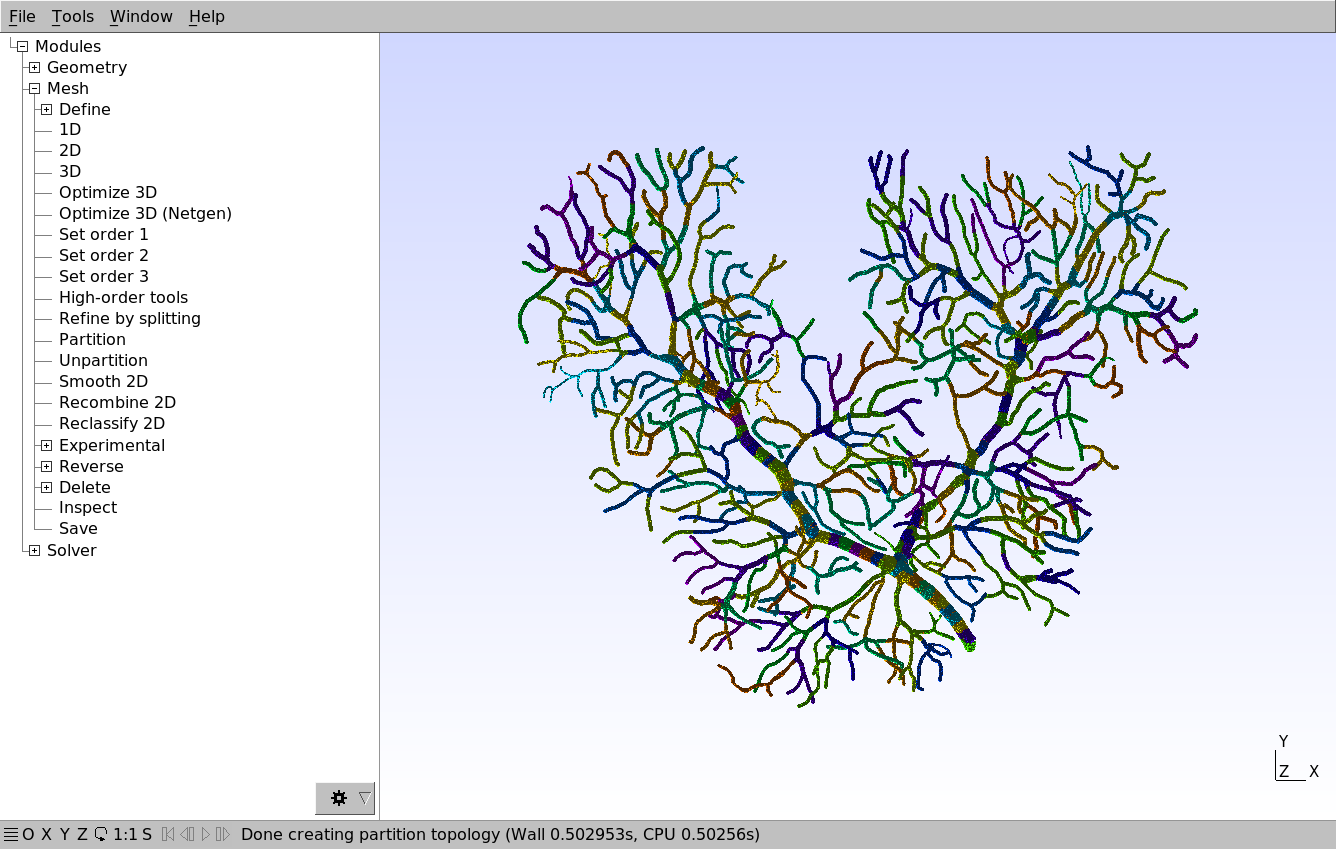
Each color represents a different partition. We then export the mesh with File \(\rightarrow\) Export…, select a destination folder and a file name ending with the .msh extension. We then make sure that “Save one file per partition” is checked in the following dialog:
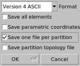
This splits the mesh into 256 distinct files suffixed with _1.msh, _2.msh, etc. The corresponding files can be downloaded from here
In STEPS, the mesh is then loaded with e.g.:
mesh = Distmesh('path/to/mesh_prefix', scale=1e-6)
We only give the part of the path that is common to all split mesh files (excluding the underscore before the partition number) and STEPS will automatically load path/to/mesh_prefix_1.msh in rank 0, path/to/mesh_prefix_2.msh in rank 1, etc. This is the method that we use in the script that we take as example in this chapter:
###########################################################
# Mesh Parameters
###########################################################

mesh_file = '../meshes/caburst_dist/split_256/CNG_segmented_2_split_256'

#...

###########################################################
# Mesh and compartmentalization
###########################################################

mesh = DistMesh(mesh_file, 1e-6)

#...
12.3. Local and global element lists
Each MPI rank loads the part of the mesh that corresponds to its partition. The elements (tetrahedrons, triangles, vertices) can then be refered to by two types of indices: a global index that uniquely identifies the element accross all MPI ranks; and a local index that is specific to each MPI rank. The following schematic shows a mesh split in two partitions along with the global (top part) and local (bottom part) indices of elements. For simplicity, we represent triangles intead of tetrahedrons but the same ideas apply to tetrahedral meshes.
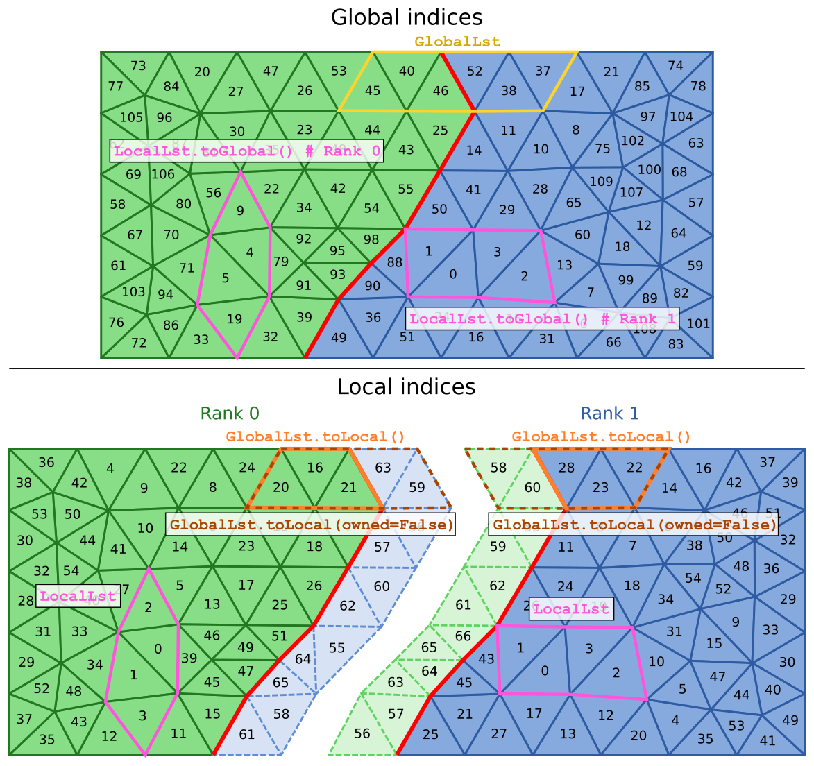
The green tetrahedrons are owned by rank 0 and the blue tetrahedrons by rank 1. The thicker red line represents the boundary between the two partitions. Note that in addition to the elements that are owned by an MPI rank (represented in darker colors and solid borders), each MPI rank also contains a shell of non-owned (or “ghost”) elements (represented in lighter colors and dashed borders) at the partition boundary. These non-owned elements share vertices with owned elements but are owned by a different MPI rank. These non-owned elements are required for synchronizing diffusion events across partition boundaries.
As can be seen on the schematic, the global and local indices are in general different and it is thus important to keep track of whether a list of elements contains indices that are global or local to the MPI rank. By default, to ensure compatibility with code written for non-distributed TetMesh meshes, all element lists are created as global lists. We can thus create the GlobalLst list that is represented on the top part of the schematic (solid yellow borders) with:
with mesh:
    GlobalLst = TetList([45, 40, 46, 52, 38, 37])
The indices that we give are the global element indices, and both rank 0 and rank 1 hold the same list that refers to the same elements.
To specify that a list is created from local indices, all lists of elements can be given an additional local keyword parameter. So we can declare the LocalLst list that is represented on the bottom part of the schematic (solid pink borders) with:
with mesh:
    LocalLst = TetList([0, 1, 2, 3], local=True)
Note that although both ranks execute the same code and display the same value of LocalLst.indices, the list refers to different mesh elements in rank 0 and rank 1.
12.3.1. Local / global conversions
We can convert the local list to its global counterpart with localLst.toGlobal():
Variable |
Rank 0 |
Rank 1 |
|---|---|---|
|
|
|
|
|
|
Although the local and global indices of some elements (like localLst in rank 1 here) can be identical, global and local indices are in general different.
Converting a local list to global is always guaranteed to return a list that has the same number of elements. However, the reverse conversion from global to local, done with e.g. GlobalLst.toLocal(), will discard the elements that are not owned by the MPI rank in which the conversion occurs. The corresponding local lists are shown in the bottom part of the schematic (solid orange border).
If the toLocal method is given an owned=False keyword parameter, the returned list will also include elements that are local to the MPI rank but which are not owned by it. These lists are represented with dashed brown borders on the schematic.
Variable |
Rank 0 |
Rank 1 |
|---|---|---|
|
|
|
|
|
|
|
|
|
Depending on whether we include non-owned elements (owned=False), the number of elements in local lists can be different. In general, we only need to consider non-owned elements when declaring compartments or patches from local lists of elements. In that case, non-owned elements are necessary so that each MPI rank can know whether diffusion can occur to the elements in other MPI ranks.
Since the toLocal method can change the number of elements in the list, when the elements are shared across several MPI ranks, we cannot recover the original global list by calling toGlobal. GlobalLst.toLocal() basically distributes its elements to the MPI ranks that owned them. We can however recover the original list with the combineWithOperator method:
import operator

with mesh:
    lst = TetList([45, 40, 46, 52, 38, 37])
    lst_local = lst.toLocal()

    lst_local_global = lst_local.toGlobal()
    lst_merge = lst_local.combineWithOperator(operator.or_)
This code results in the following values:
Variable |
Rank 0 |
Rank 1 |
|---|---|---|
|
|
|
|
|
|
|
|
|
|
|
|
Calling the combineWithOperator method allows us to recover the original global list. This method takes a binary operator that should combine two lists into a merged list, this operator gets repeatedly applied to create the merged list. Any function that takes two global lists and returns a global list can be given to combineWithOperator but most of the time, it is easier to use one of the binary operator functions in the operator
python package. Here we use operator.or_, which corresponds to the | operator that we would normally use to combine lists (see the corresponding chapter).
In order to determine whether a given element list is local, one can call the isLocal method.
12.3.2. Using the mesh locally
Element lists that are directly accessed through the mesh or its components (compartments, patches, membranes, etc.) are global lists by default. To avoid the MPI synchronization necessary to obtain these global lists, it is possible to use the asLocal method with the following syntax:
with mesh.asLocal():
    localTets = mesh.tets
As long as we are in the with mesh.asLocal(): block, mesh properties will be local by default. The same thing applies to mesh components like compartments, etc. Note that with mesh.asLocal(): does not change whether lists created in the block will be global or local, the local keyword argument should still be provided to all lists that are explicitely created, and global lists can still be used in a with mesh.asLocal(): block.
Like for toLocal, the asLocal method can take an owned keyword argument that defaults to True so the above code only considers owned elements. To consider non-owned elements as well, one would write:
with mesh.asLocal(owned=False):
    allLocalTets = mesh.tets
This is usually not needed, except when declaring compartments or patches from lists of local elements. As we saw earlier, non-owned elements are necessary for diffusion and since diffusions operate within compartments / patches, each MPI rank needs to know whether its non-owned elements are part of the same compartment / patch as its owned elements.
Finally, when using distributed meshes, it is advisable to use with mesh.asGlobal(): instead of with mesh:. They have the same effect since the mesh is in global mode by default, but the former makes it clearer which parts of the code use the mesh globally.
12.5. Creating compartments and patches
12.5.1. Compartments
Going back to our main example, we first create the cyto compartment. This compartment will contain all the tetrahedrons in the mesh and will thus be created from the mesh.tets list. We could declare it as we would in a 'TetOpSplit' simulation, using global indices:
with mesh:
    cyto = Compartment.Create(mesh.tets, vsys)
    # ...
The issue with this code, however, is that all MPI ranks will hold mesh.tets, the full list of tetrahedrons in the whole mesh. Since the goal of a distributed simulation is to have each MPI rank only consider tetrahedrons that are in its partition, it is preferable to create the compartment from lists of local tetrahedrons.
We thus use the mesh.asLocal(owned=False) syntax we saw in the previous section:
with mesh.asLocal(owned=False):
    cyto = Compartment.Create(mesh.tets, vsys)
    cyto.Conductivity = 1 / Ra
Since we are in a with mesh.asLocal(owned=False): block, mesh.tets returns a local list incuding non-owned elements.
With the 'Tetexact' and 'TetOpSplit' solvers, the volume resistivity Ra (in Ohm.m) is set for the membrane object after simulation creation (by calling e.g. sim.membrane.VolRes = Ra, see the calcium burst chapter). The 'DistTetOpSplit' distributed solver instead requires setting the volume conductivity (in S/m) of compartments before the simulation. We thus set the
Conductivity property to the reciprocal of the resistivity Ra. Note that we could also give the conductivity keyword argument upon creation of the compartment: cyto = Compartment.Create(mesh.tets, vsys, conductivity=1 / Ra). If the keyword argument is not supplied and the Conductivity property not set, its value defaults to 0.
12.5.2. Patches
We want to create two patches that correspond to the spiny and smooth parts of the mesh surface. Since the tags in the mesh files are associated with tetrahedrons and not triangles, we first need to get the local lists of 'spiny' and 'smooth' tetrahedrons. We then compute the surface of these local lists and intersect it with the surface of the mesh:
with mesh.asLocal(owned=False):
    #...

    smoothTets = mesh.tetGroups['smooth']
    spinyTets = mesh.tetGroups['spiny']

    smooth = Patch.Create(smoothTets.surface & mesh.surface, cyto, None, ssys)
    spiny = Patch.Create(spinyTets.surface & mesh.surface, cyto, None, ssys)
The patch creation is exactly the same as for 'Tetexact' or 'TetOpSplit' simulations, we provide the list of elements (here a local list that also includes non-owned elements), the inner compartment (cyto), the outer compartment (which is absent here) and the associated surface system.
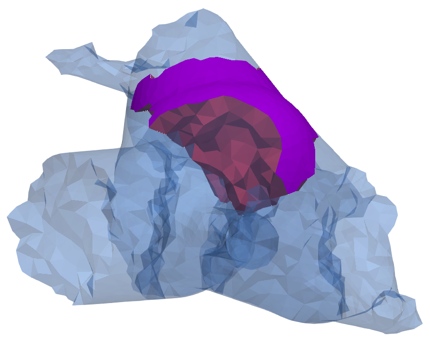
The local list of triangles that is given is obtained by first computing the surface of the list of local tetrahedrons (in red and purple in the figure below) with e.g. smoothTets.surface (see the documentation of the surface property). We then compute the intersection between this surface and the surface of the mesh to get rid of the internal surface that corresponds to the partition boundaries (the red part). The resulting surface is
represented in purple in the figure below:
12.5.4. Membranes
Finally, we create the smooth and spiny membranes with:
with mesh.asLocal(owned=False):
    #...

    memb_smooth = Membrane.Create([smooth], capacitance=memb_capac_proximal)
    memb_spiny = Membrane.Create([spiny], capacitance=memb_capac_spiny)
Note that, in contrast with membrane creation for the TetOpSplit solver, we need to create one membrane per patch and give the membrane capacitance before the simulation. Alternatively, we could have set the membrane capacitance with the Capacitance property:
with mesh.asLocal(owned=False):
    #...

    memb_smooth = Membrane.Create([smooth])
    memb_spiny = Membrane.Create([spiny])

    memb_smooth.Capacitance = memb_capac_proximal
    memb_spiny.Capacitance = memb_capac_spiny
12.6. Distributed mesh simulation
As mentionned before, we will use the distributed 'DistTetOpSplit' solver, so the simulation object is created like so:
###########################################################
# Simulation
###########################################################

rng = RNG('mt19937', 512, SEED)

sim = Simulation(
    'DistTetOpSplit', mdl, mesh, rng,
    searchMethod=NextEventSearchMethod.GIBSON_BRUCK
)
The main difference from 'Tetexact' or 'TetOpSplit' is that we do not need to provide the Efield flag that determines whether membrane potential should be computed (see corresponding chapter; and we do not need to provide a partition object (see corresponding chapter. In addition, we set the searchMethod keyword argument to the Gibson
Bruck method. Although a different direct method is also implemented, we currently recommend to always explicitely use the Gibson Bruck method when using 'DistTetOpSplit'.
12.6.1. Data saving
We then declare the data that should be saved:
with mesh.asLocal():
    Pots = rs.VERTS(mesh.surface.verts).V
    CaConc = rs.TETS().Ca.Conc
    CaConc.metaData['Vols'] = [tet.Vol for tet in mesh.tets]
    Currents = rs.TRIS(mesh.surface).OC_CaP.I

sim.toSave(Pots, CaConc, Currents, dt=DT)
Since we are using a distributed solver, the data to be saved should also preferentially be local to avoid the creation of global element lists. We thus declare the result selectors inside a with mesh.asLocal(): block so that mesh.surface.verts and mesh.surface return local lists of elements. We save the membrane potential over all mesh surface vertices, the calcium concentration in all tetrahedrons, and the calcium GHK currents over all surface triangles. Note that we also record
the volume of each tetrahedrons in the CaConc metadata (see corresponding section) so that we can later recover the quantities of Ca in each tetrahedron.
We then use the XDMFHandler database class that we introduced in a previous chapter:
with XDMFHandler('DistCaburst') as hdf:
    sim.toDB(hdf, 'CaBurstSim')

    sim.newRun()

    # Initial state setting...
    # Run loop...
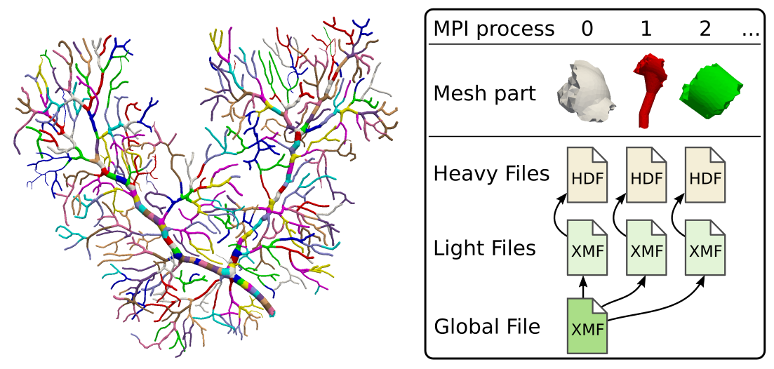
The XDMFHandler class is necessary to take advantage of distributed data saving. Instead of creating a single HDF5 file along with its associated XDMF file, it will create one HDF5 and XDMF file per MPI rank as well as a global XDMF file that contains references to the partitions’ XDMF files:
12.6.2. Running the simulation
We run the simulation in the same way as for parallel simulations:
mpirun -n 256 python3 STEPS_Tutorial_Distributed.py
Note that, for technical reasons, the number of ranks must be a power of 2. The full simulation is most likely too big to be run on a personnal computer and should instead be run on a computing cluster.
However, since the mesh is distributed, it is possible to run the simulation for a smaller subpart of the mesh. We can for example run it on the first 4 mesh parts with:
mpirun -n 4 python3 STEPS_Tutorial_Distributed.py
Since only 4 out of the 256 parts are loaded, this can definitely be run on a personnal computer. Note that the results we would obtain from such a simulation are not necessarily biologically relevant since we are changing the ratio of smooth to spiny dendrite surface.
12.7. Data visualization
The saved data can be visualized in Paraview as presented in the data recording and analysis chapter by opening the CaBurstSim_Run0_Full.xmf file. The data for each MPI rank can also be loaded separately by opening e.g. CaBurstSim_Run0_rank0.xmf. Paraview usage is however beyond the scope of this chapter and interested readers should consult the Paraview user guide.
As an illustration, here is an example of visualization of intracellular calcium concentrations in a simulation that was run using only the first 4 parts of the mesh (as shown in the previous section):
The simulation can be played by opening the menu, switching to the “GLOBAL” tab, and clicking on the Play button.
Here are examples of Paraview usage and figures made with the data from the full mesh simulation and 3D snapshots of membrane potential and tetrahedron calcium concentration at 8ms: 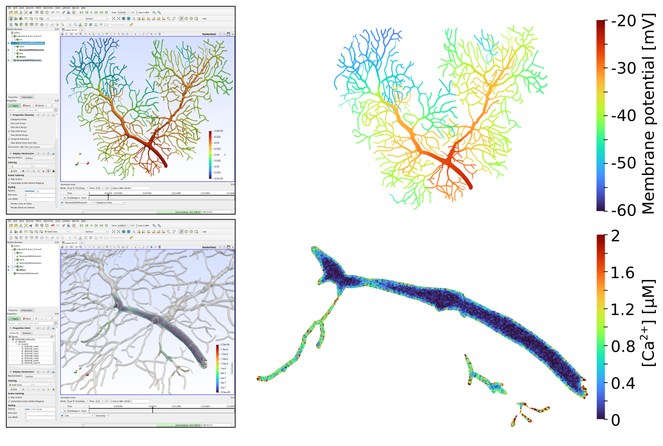
12.8. Data loading in python
The data that we recorded can also be loaded in python with the HDF5Handler class. STEPS will automatically open the individual .h5 files corresponding to each MPI rank and the results will be accessible as if everything was saved in a single file.
For example, we can plot average values with:
[1]:
import steps.interface

from steps.saving import *

from matplotlib import pyplot as plt
import numpy as np

with HDF5Handler('scripts/DistCaburst') as hdf:
    Pots, CaConc, Currents = hdf['CaBurstSim'].results

    plt.figure(figsize=(10,7))
    plt.plot(Pots.time[-1], 1e3 * np.mean(Pots.data[-1], axis=1))
    plt.xlabel('Time [s]')
    plt.ylabel('Membrane Potential [mV]')
    plt.show()

    plt.figure(figsize=(10,7))
    vols = CaConc.metaData['Vols']
    mols = CaConc.data[-1] * vols
    plt.plot(Pots.time[-1], 1e6 * np.sum(mols, axis=1) / sum(vols))
    plt.xlabel('Time [s]')
    plt.ylabel('Intracellular calcium concentration [uM]')
    plt.show()

    plt.figure(figsize=(10,7))
    plt.plot(Pots.time[-1], 1e9 * np.sum(Currents.data[-1], axis=1))
    plt.xlabel('Time [s]')
    plt.ylabel('CaP current [nA]')
    plt.show()
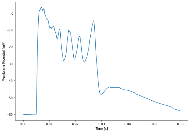
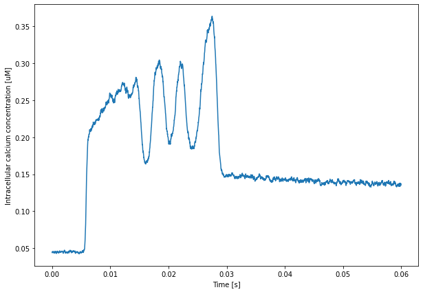
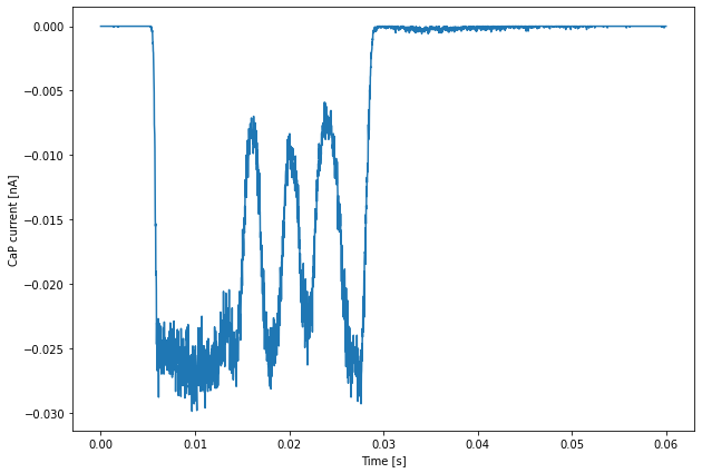
The data for these plots has been obtained using the restricted 4 rank run that we discussed previously.