4. Surface-Volume Reactions

Topics: Surface reactions, chained reactions, advanced ResultSelector usage.

The corresponding python script: STEPS_Tutorial_IP3.py

In the previous chapter we declared reactions taking place inside a volume. In this chapter we consider another type of kinetic reaction, associated with the steps.model.SurfaceSystem container, which defines a reaction taking place on a surface (or patch) connecting two compartments (arbitrarily naming one of them the “inner” compartment, and the other one the “outer” compartment). Reactants and products can therefore be freely moving around in a volume or embedded in a surface. Therefore, it is necessary to firstly specify the location of the reactant and product species.

Note: Surface reactions are designed to represent reactions where one reactant is embedded in a membrane, but in fact if all reactants and products belong to the same compartment and none appear on a patch it will behave exactly like the equivalent volume reaction.

To become familiar with these reactions we will build a simplified version of the inositol 1,4,5-trisphosphate (IP \(_{3}\)) model (described in Doi T, et al,Inositol 1,4,5-Triphosphate-Dependent \(Ca^{\text{2+}}\) Threshold Dynamics Detect Spike Timing in Cerebellar Purkinje Cells, J Neurosci 2005, 25(4):950-961) in STEPS.

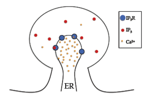
In the IP3 receptor model, reactions (i.e. receptor binding of calcium and IP3 molecules) take place on the membrane separating the Endoplasmic Reticulum (ER) and the cytosol. Therefore, we will need to declare surface reactions.

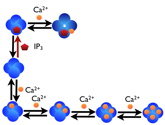
In the figure below we can see a schematic diagram of the states and transitions in the model. IP3 receptors are embedded in the ER membrane, each “binding” reaction is described by a second order surface reaction and each “unbinding” reaction by a first order surface reaction.

We will go through the Python code to build this model in STEPS, but providing only brief descriptions of operations we are familiar with from the previous chapter.

4.1. Model declaration

4.2. Surface reactions

STEPS surface reactions can deal with three types of reactions, classified by the locations of the reactants:

• Volume-Surface reactions. In this case molecules within a volume interact with molecules embedded in a surface and result in products that may reside within in a volume or a surface. The units for the reaction parameters in this case are the same as for ordinary volume reactions, namely: a first order reaction parameter has units \(s^{-1}\); a second order reaction parameter has units \(\left(M.s\right)^{-1}\); a third order reaction \(\left(M^{2}.s\right)^{-1}\); and so on.

• Surface-Surface reactions. In this case the reactants are all embedded in a surface. Quite clearly, the dimensions of the reaction are different from a volume reaction and the reaction parameter is assumed to be two-dimensional. This is an important point because the reaction parameter will be treated differently from a volume-volume or volume-surface interaction. A further complication is that parameters for ordinary volume reactions are based on the litre, where there is no convenient equivalent 2D concentration unit. Surface-surface reaction parameters are based on units of area of square meters. A first order surface-surface reaction parameter is therefore required in units of \(s^{-1}\); a second-order surface-surface reaction parameter has units \(\left(mol.m^{-2}\right)^{-1}.s^{-1}\); a third-order surface-surface reaction parameter has units \(\left(mol.m^{-2}\right)^{-2}.s^{-1}\); and so on. Zero-order surface reactions are not supported because of the ambiguity of interpreting the reaction parameter.

• Volume-Volume reactions. It is possible for a surface reaction to contain reactant species that are all in a volume, in which case the reaction behaves similarly to an ordinary volume reaction, though products may belong to connected volumes or surfaces.

As mentioned previously, to declare surface reactions we have to include some information about the location of the reaction: which compartment are the reactants to be found in, and are any molecules embedded in a surface and which of the two compartments that the surface connects are the products injected into? We supply this information to STEPS by labelling our compartments that a patch connects, arbitrarily choosing the labels ‘inner’ and ‘outer’. When the surface reaction’s parent surface system object is added to a certain patch, the compartment labelling in the surface reaction stoichiometry will match the compartment labelling in the patch definition. We will come to creating a patch later in this chapter.

So, at this stage we must chose which compartment we will label ‘outer’ and which we will label ‘inner’ and make sure to maintain this labelling throughout our definitions, and also in our geometry description. We chose to label the cytosol as the ‘outer’ compartment and the ER as the ‘inner’ compartment, so should be very careful that this ties in correctly to our description when we create our steps.geom.Patch object to represent a surface to connect the two compartments.

When writing a surface reaction, we can specify the location of each reactant in two different ways. The most verbose consist in using functions In, Out and Surf to refer respectively to the inner compartment, the outer compartment, and the patch surface:

Surf(R) + Out(IP3) <r[1]> Surf(RIP3)

The same reactions can be declared in a slightly more concise way:

R.s + IP3.o <r[1]> RIP3.s

Adding .s, .i, or .o after a reactant is a shorthand way to specify its location. This notation aims at imitating subscripts like in: \(\mathrm{R_s + IP3_o \leftrightarrow RIP3_s}\)

Note: Reactant species cannot belong to different compartments, so attempting to create a surface reaction with both Spec1.i and Spec2.o will result in an error.

4.3. Surface reactions declaration

Let us now declare all our reactions. As in the previous chapter, we first import the required packages, create the Model, a ReactionManager, and declare Species:

import steps.interface

from steps.model import *
from steps.geom import *
from steps.rng import *
from steps.sim import *
from steps.saving import *

r = ReactionManager()

mdl = Model()

with mdl:
    Ca, IP3, R, RIP3, Ropen, RCa, R2Ca, R3Ca, R4Ca = Species.Create()
    surfsys = SurfaceSystem.Create()

    with surfsys:
        # IP3 and activating Ca binding
        R.s    + IP3.o <r['r1']> RIP3.s
        RIP3.s + Ca.o  <r['r2']> Ropen.s
        r['r1'].K = 1000e6, 25800
        r['r2'].K = 8000e6, 2000

        # Inactivating Ca binding
        R.s    + Ca.o <r['r3']> RCa.s
        RCa.s  + Ca.o <r['r4']> R2Ca.s
        R2Ca.s + Ca.o <r['r5']> R3Ca.s
        R3Ca.s + Ca.o <r['r6']> R4Ca.s
        r['r3'].K = 8.889e6, 5
        r['r4'].K = 20e6, 10
        r['r5'].K = 40e6, 15
        r['r6'].K = 60e6, 20

        # Ca ions passing through open IP3R channel
        Ca.i + Ropen.s >r[1]> Ropen.s + Ca.o
        r[1].K = 2e8

Note that each possible state of an IP3 receptor is declared as a dinstinct species. We then declare a SurfaceSystem instead of a VolumeSystem and the reactions are declared using the context manager with keyword, as previously seen. All reactions are reversible (using <r[...]>) except for the last one (using >r[...]>), that represents calcium leaving the ER through the open IP3R channel.

By using the .K property, we set all reaction constants’ default values (see Doi T, et al,Inositol 1,4,5-Triphosphate-Dependent \(Ca^{\text{2+}}\) Threshold Dynamics Detect Spike Timing in Cerebellar Purkinje Cells, J Neurosci 2005, 25(4):950-961). Since these are volume-surface interactions, we must make sure to supply our values in Molar units as discussed previously in this chapter.

Note that, when several reactants bind sequentially (to a receptor like here for example), it is possible to chain the reactions using parentheses:

(R.s + IP3.o <r[1]> RIP3.s) + Ca.o <r[2]> Ropen.s

Reactions that are in parentheses are equivalent to their right hand side. The above line thus first declares the reaction in the parentheses R.s + IP3.o <r[1]> RIP3.s and replaces it by its right hand side; the line then reads RIP3.s + Ca.o <r[2]> Ropen.s and this reaction is declared. The whole process is thus equivalent to declaring the reactions on two separate lines.

Warning: Chained reactions can be a bit hard to read so their use should probably be restricted to sequential bindings.

4.4. Geometry specification

The next step is to create the geometry for the model. We will choose well-mixed geometry, as in the chapter on well-mixed models, but we now have two compartments which are connected by a surface ‘patch’. We create two steps.geom.Compartment objects to represent the Endoplasmic Reticulum (which we intend to label the ‘inner’ compartment) and the cytosol (‘outer’ compartment), and a steps.geom.Patch object to represent the ER membrane between the ER and cytosol.

geom = Geometry()
with geom:
    # Create the cytosol and Endoplasmic Reticulum compartments
    cyt, ER = Compartment.Create()
    cyt.Vol = 1.6572e-19
    ER.Vol = 1.968e-20

    # ER is the 'inner' compartment, cyt is the 'outer' compartment
    memb = Patch.Create(ER, cyt, surfsys)
    memb.Area = 0.4143e-12

First we create the two well-mixed compartments at once with cyt, ER = Compartment.Create(). Since no parameters were given to Create(), we explicitely set the volume of each compartment by using the .Vol property. Since we only defined a SurfaceSystem in the model, we do not need to associate our compartment with a VolumeSystem.

We then create the Patch using the automatic naming syntax. This time, the Create method needs to receive at least the inner compartment. It is vital that care is taken in the order of the compartment objects to the constructor, so that the required labelling from our surface reaction definitions is maintained. Note: A Patch must have an inner compartment by convention, but does not require an outer compartment. This is an easy way to remember the order to the constructor; since an inner compartment is always required it must come first to the constructor, and the optional outer compartment comes after. Obviously any surface reaction rules that contain reactants or products in the outer compartment cannot be added to a Patch that doesn’t have an outer compartment.

We can also specify the area of the patch during creation, like so:

patchName = Patch.Create(innerComp, outerComp, surfSys, area)

In our example, we set the area of a patch after creation using the .Area property.

We can check the labelling is as desired after object construction if we like with properties steps.geom.Patch.innerComp and steps.geom.Patch.outerComp.:

print(memb.innerComp)
print(memb.outerComp)

ER
cyt

4.5. Simulation declaration and data saving

We first create the random number generator and the Simulation. Like in the previous chapter, we will use the well-mixed 'Wmdirect' solver:

rng = RNG('mt19937', 512, 7233)

sim = Simulation('Wmdirect', mdl, geom, rng)

Model checking:
No errors were found

We then specify which data should be saved, this time we will declare two result selectors:

rs = ResultSelector(sim)

Rstates = rs.memb.MATCH('R.*').Count

Reacs = rs.memb.MATCH('r[1-6]')['fwd'].Extent + rs.memb.MATCH('r[1-6]')['bkw'].Extent

We have two ResultSelectors, Rstates and Reacs. Rstates makes use of the MATCH(...) function that only selects objects whose name matches the regular expression given as a parameter. In our case, it will match all objects inside memb whose name starts with ‘R’, i.e. all receptors. It is equivalent to the longer:

Rstates = rs.memb.LIST(R, RIP3, Ropen, RCa, R2Ca, R3Ca, R4Ca).Count

In our specific case, it happens to be equivalent to rs.memb.ALL(Species).Count because we did not define any other species on the ER membrane. The MATCH version is however preferable since it will still work if we decide to add other species.

4.5.1. Combining ResultSelectors

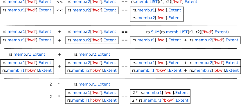
The second ResultSelector, Reacs will save the extent of each reaction from ‘r1’ to ‘r6’, taking into account both forward and backward subreactions. To understand its declaration, we first need to see how reactions interact with ResultSelectors. The following ResultSelector will save both forward and backward extent of reaction ‘r1’:

rs.memb.r1.Extent

Since it saves two values for each run and for each timestep (i.e. the third dimension of the associated data structure is 2, cf. previous tutorial), and for the sake of simplicity, we will say that it has length 2. To save specifically the forward extent, we write:

rs.memb.r1['fwd'].Extent

and this ResultSelector has length 1. To save the total extent (the sum of forward and backward), one could write:

rs.SUM(rs.memb.r1.Extent)

the rs.SUM(...) function takes a ResultSelector as an argument and returns a ResultSelector whose length is 1 and corresponds to the sum of all the values defined by the argument. In our case, it would be equivalent to:

rs.memb.r1['fwd'].Extent + rs.memb.r1['bkw'].Extent

This + notation is also valid; standard arithmetic operators (+, -, *, /, and **) can all be used with ResultSelectors and behave in the same way as they do in numpy. The above example sums two ResultSelectors of length 1 and thus results in a ResultSelector of length one as well. If the length of the operands is higher than one, like in:

rs.memb.LIST(r1, r2)['fwd'].Extent + rs.memb.LIST(r1, r2)['bkw'].Extent

the resulting ResultSelector has length 2, like the operands, and is equivalent to:

rs.memb.r1['fwd'].Extent + rs.memb.r1['bkw'].Extent << rs.memb.r2['fwd'].Extent + rs.memb.r2['bkw'].Extent

In our main example, Reacs has length 6 and saves the total extent of each reaction whose name matches the regular expression ‘r[1-6]’ (the name has to start with character ‘r’ and then a number between 1 and 6).

4.5.2. Editing labels

As we saw in the previous tutorial, labels are automatically generated when using ResultSelectors and can be accessed with e.g. Rstates.labels. With the same notation, it is also possible to provide custom labels by simply using:

selector.labels = ['label 1', 'label2', ...]

The length of the list needs to match the length of the ResultSelector. Here, we will modify the automatically generated labels of Rstates which currently look like this:

print(Rstates.labels)

['memb.R.Count', 'memb.R2Ca.Count', 'memb.R3Ca.Count', 'memb.R4Ca.Count', 'memb.RCa.Count', 'memb.RIP3.Count', 'memb.Ropen.Count']

Instead, we would like to only keep the species name:

Rstates.labels = [l.split('.')[1] for l in Rstates.labels]

print(Rstates.labels)

['R', 'R2Ca', 'R3Ca', 'R4Ca', 'RCa', 'RIP3', 'Ropen']

4.5.3. Data saving

As previously, we associate both ResultSelectors to the simulation and specify how frequently they should be saved:

sim.toSave(Rstates, Reacs, dt=0.001)

If the results needed to be saved at different intervals, we could of course write:

sim.toSave(Rstates, dt=0.001)
sim.toSave(Reacs, dt=0.005)

In addition, if we wanted to save the data at specified timepoints, we could use the timePoints argument:

sim.toSave(Reacs, timePoints=[0.0, 0.01, 0.03, 0.15])

4.5.4. Running the simulation

Having defined and added all ResultSelectors, we can then run the simulation:

NITER = 100
ENDT = 0.201

for i in range (0, NITER):
    sim.newRun()

    sim.cyt.Ca.Conc = 3.30657e-8
    sim.cyt.IP3.Count = 6
    sim.ER.Ca.Conc = 150e-6
    sim.ER.Ca.Clamped = True
    sim.memb.R.Count = 160

    sim.run(ENDT)

4.6. Plotting the results

We first plot the number of open IP3 receptors as a function of time:

from matplotlib import pyplot as plt
import numpy as np

plt.figure(figsize=(10, 7))

RopenInd = Rstates.labels.index('Ropen')
RopenData = Rstates.data[:, :, RopenInd]

time = Rstates.time[0]
mean = np.mean(RopenData, axis=0)
std = np.std(RopenData, axis=0)

plt.plot(time, mean, linewidth=2, label='Average')
plt.fill_between(time, mean - std, mean + std, alpha=0.2, label='Std. Dev.')

for t, d in zip(Rstates.time, RopenData):
    plt.plot(t, d, color='grey', linewidth=0.1, zorder=-1)

plt.ylim(0)
plt.margins(0, 0.05)
plt.xlabel('Time [s]')
plt.ylabel('Number of open IP3R')
plt.legend()
plt.show()

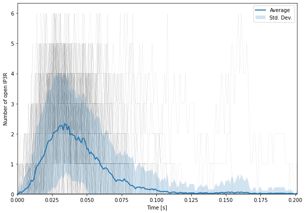
We first need to extract the data for Ropen from Rstates. We do so by using Rstates.labels; we are interested in memb.Ropen.Count so we simply call the python index method that returns the index of the Ropen data in the whole selector. We then get the corresponding data with Rstates.data[:, :, RopenInd], the two first dimensions (runs and time) are untouched and we only take the data relative to Ropen.

In order to display the trace corresponding to each run, we iterate on the data with:

for t, d in zip(Rstates.time, RopenData):
    plt.plot(t, d, color='grey', linewidth=0.1, zorder=-1)

We would then like to look at the time course of all receptor states:

plt.figure(figsize=(10, 7))

time = Rstates.time[0]
mean = np.mean(Rstates.data, axis=0)
std = np.std(Rstates.data, axis=0)

plt.plot(time, mean, linewidth=2)
for m, s in zip(mean.T, std.T):
    plt.fill_between(time, m - s, m + s, alpha=0.2)

plt.legend(Rstates.labels)
plt.xlabel('Time [s]')
plt.ylabel('Number of receptors')
plt.ylim(0)
plt.margins(0, 0.05)
plt.show()

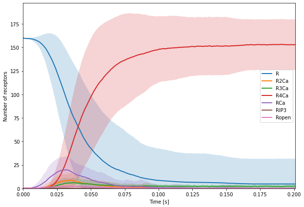
Since fill_between cannot take all data at once, like plot can, we needed to iterate over the different receptor states in mean and std. To do so, we used:

for m, s in zip(mean.T, std.T):
    plt.fill_between(time, m - s, m + s, alpha=0.2)

both mean and std have dimension (nbT, nbR) with nbT the number of saved time points and nbR the number of receptor states. Since the first dimension corresponds to time, if we were to directly iterate over mean and std, we would iterate over time instead of iterating over receptor states. We thus first transpose the matrices with mean.T and std.T.

We then turn to plotting data from Reacs:

plt.figure(figsize=(10, 7))

time = Reacs.time[0]
dt = time[1] - time[0]
meanDeriv = np.mean(np.gradient(Reacs.data, dt, axis=1), axis=0)

plt.stackplot(time, meanDeriv.T)

plt.legend([f'd{l} / dt' for l in Reacs.labels])
plt.margins(0, 0.05)
plt.xlabel('Time [s]')
plt.ylabel('Total reaction rate [1/s]')
plt.show()

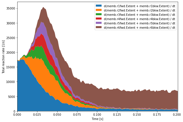
Here we want to look at the repartition of the actual rates of reactions. We use the np.gradient function that computes the derivative of the data with respect to the time axis (axis=1). We then average the values across runs using np.mean with axis=0. This time derivative of the extent of each reaction is a good proxy for the instantaneous actual rate of this reaction.